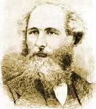
The aim of exact science is to reduce the problems of nature to the
determination of quantities by operations with numbers. James Clerk Maxwell
(1831-1879) On Faraday's Lines of Force (1856)
The following modern presentation of electromagnetism incorporates three
clarifications which came only many years after
Maxwell's original work (1864):
Arguably, the original equations of Maxwell (1864) were essentially
the so-called macroscopic equations,
which describe electromagnetism in a dense medium.
The microscopic approach (which is now standard)
is due to
H.A. Lorentz (1853-1928).
Lorentz showed how the introduction of
densities of
polarization and magnetization
reduces the macroscopic equations ("in matter") to the more fundamental
microscopic ones ("in vacuum") stated
below.
Giovanni Giorgi
Except in the first article,
we consider only one flavor
of electromagnetic quantities and use only
the MKSA units introduced by
Giovanni Giorgi
(1871-1950) in 1901, which are the basis of
all modern SI electrical units:
ampere (A), ohm (W), coulomb (C),
volt (V), tesla (T), farad (F), henry (H), weber (Wb)...
(2005-07-22)
The Former Problem with Electromagnetic Units
A science which hesitates to forget its founders is lost.
Alfred North
Whitehead
(1861-1947)
This article is of historical interest only. You are advised to
skip it
if you were blessed with an education entirely grounded
on Giorgi's electrodynamic units (SI units based on the MKSA system).
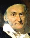
The first consistent system of mechanical units was the
meter-gram-second system advocated by Carl
Friedrich Gauss in 1832.
It was used by Gauss and Weber (c.1850)
in the first definitions of electromagnetic units in absolute terms.
However, the term Gaussian system now refers to a particular
mix of electrical C.G.S. units (discussed below) once dominant
in theoretical investigations.
James Clerk Maxwell himself was instrumental in bringing about the
cgs system in 1874 (centimeter-gram-second).
Two sets of electrical units were made part of the system.
An enduring confusion results from the fact that the quantities measured by these
different units have different definitions
(in modern terms, for example,
the magnetic quantity now denoted B could be either B or cB).
Following Maxwell's own vocabulary, it's customary to speak of either
electrostatic units (esu) or
electromagnetic units (emu).
However, one must appreciate the obscure fact that these two are not
only different system of units, they are different traditions
in which symbols may have different meanings...
At first, no C.G.S. electromagnetic units had a specific name.
On August 25th, 1900, the
International
Electrical Congress (IEC) adopted 2 names:
Gauss for the CGS unit of magnetic field
(B) :
1 G = 10 -4 T.
Maxwell for the CGS unit of magnetic flux
(F) :
1 Mx = 10 -8 Wb.
The maxwell, still known as a line of force,
is called abweber (abWb)
using the later naming of CGS electrical units after their
MKSA counterparts. Likewise, the gauss
(1 maxwell per square centimeter)
is also called abtesla (abT).
For electrostatic CGS units (esu)
the prefix stat- is used instead...
In 1930, the Advisory Committee on Nomenclature of the IEC adopted the
gilbert
(Gb) as a CGS-emu unit equal to the magnetomotive force
around the border of a surface through which flows a current of
(1/4p) abA.
The relevant values in SI units are:
1 abA = 10 A
1 Gb = (10/4p) A-t
= 0.795774715459... A-t
1 A-t = 1 A
The last expression is to say that no distinction is made in SI units between
an ampere-turn and an ampere.
Although the gilbert seems obsolete, the oersted (equal to one gilbert
per centimeter) is still very much alive
in the trade as a unit of
magnetization (density of magnetic dipole moment
per unit volume) and/or magnetic field strength (the vectorial quantity
usually denoted H).
The oersted
was introduced by the IEC in the plenary convention at Oslo, in 1930.
Electrodynamic units are now based on a proper independent electrical unit,
as advocated by the Italian engineer Giovanni Giorgi (1871-1950) in 1901:
The addition of the ampère to the MKS system has turned it
into a consistent 4-dimensional system (MKSA)
which is the foundation for modern SI units.
Paradoxically, this mess comes from a great clarification of Maxwell's:
The ratio of the emu value to the esu value of a given field
is equal to the speed of light
(c = 299792458 m/s).
Scholars from bygone days should be credited
for accomplishing so much in spite of such confusing systems.
(2005-07-15)
The Lorentz Force
The Lorentz force on a test particle defines
the electromagnetic field(s).
The expression of the Lorentz force introduced here defines dynamically the fields
which are governed by Maxwell's equations,
as presented further down.
Neither of these two statements is a logical consequence of the other.
Such a definition is anachronistic:
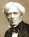
The concept of an electromagnetic field is due to
Michael Faraday (1791-1867) while
the modern expression of the force exerted by electromagnetic fields on a moving
electric charge was devised in 1892 by
H.A. Lorentz (1853-1928).
In electrostatics, the electric field E
present at the location of a particle of charge q
summarizes the influence of all other electric charges, by stating that
the particle is submitted to an electrostatic force equal to q E.
This defines E.
This concept may be extended to
magnetostatics for a moving test particle.
More generally, the electromagnetic fields need not be
constant in the following expression of the force acting on a particle of charge
q moving at velocity v.
The Lorentz Force (1892)
F =
q ( E + v´B )
The average force exerted per unit of volume may thus be expressed in terms of
the density of charge r
and the density of currentj.
Density of Force
dF / dV
=
r E +
j ´ B
Another way to define the
magnetic fieldB
(best called "magnetic induction")
would involve the concept of a pointlike
magnetic dipole.
Today, this may look less elementary than the previous method,
but this is the way B could readily be quantified by Coulomb,
using the same torsion balance he used in the celebrated investigations
of electrostatics (1785)
presented in the next section...
Torque on a Magnetic Dipolem
m ´ B
Potential Energy of a Dipolem
- m . B
The force exerted on a dipole
is grad (m.B).
It vanishes in a uniform field.
(2005-07-18)
Electrostatics:
On the electric field from static charges.
Coulomb's inverse square law
translates into the local differential property of the field expressed by Gauss,
namely: div E = r/eo
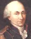
The SI unit of electric charge is named after the French military engineer
Charles
Augustin de Coulomb (1736-1806). Using a torsion balance,
Coulomb discovered, in 1785, that the
electrostatic
force between two charged particles is proportional to each charge,
and inversely proportional to the square of the distance between them.
In modern terms, Coulomb's Law reads:
Electrostatic Force
between Two Charged Particles
|| F || =
| qq' |
4peo r 2
The coefficient of proportionality denoted 1/4peo
(to match the modern conventions about the rest of electromagnetism)
is called Coulomb's constant and is roughly equal to 9 109
if SI units are used (forces in newtons,
electric charges in coulombs and distances in meters).
More precisely, the modern definitions of the units of electricity
(ampere) and distance (meter)
give Coulomb's constant an exact value in SI units whose digits are the
same as the square of the speed of light (itself exactly equal to 299792458 m/s
because of the way the meter is defined nowadays):
1
=
8.9875517873681764 ´ 10 9 m / F
» 9 ´ 10 9
N . m 2 / C 2
4peo
The direction of the electrostatic force
is on the line joining the two charges.
The force is repulsive
between charges of the same sign (both negative or both positive).
It's attractive between charges of unlike signs.
In the language of fields introduced above,
all of the above is summarized by the following
expression, which gives the electrostatic field E
produced at position r by a motionless particle of charge q
located at the origin:
Electrostatic Field of aPoint Charge at the Origin
E =
qr
4peo r 3
Since r / r 3
is the opposite of the gradient of 1/r,
we may rewrite this as :
E =
- grad f
where f
=
q
4peo r
The additivity of forces means that the contributions to the local field E
of many remote charges are additive too.
The electrostatic potential
f we just introduced may thus be computed additively as
well. This leads to the following formula, which reduces the computation of
a three-dimensional electrostatic field to the integration
of a scalar
over any static distribution of charges:
The Electrostatic Field Eand Scalar Potential f
E =
- grad f
where f(r)
=
òòò
r(s)
d3s
4peo
|| r - s ||
The above static expression of E would have to be
completed with a dynamic quantity (namely
-¶A/¶t,
as discussed below)
in the nonstatic case governed by the full set of
Maxwell's equations.
Also, the dynamical scalar potential
f involves a
more delicate integration than the above one.
In 1813, Gauss bypassed
both dynamical caveats with a local differential expression,
also valid in electrodynamics :
div E =
r
eo
A similar differential relation had been obtained by Lagrange
in 1764 for Newtonian gravity
(which also obeys an inverse square law).
This can be established with elementary methods...
One way to do so is to approximate any distribution of charges
by a sum of pointlike sources: For each point charge q,
we can check that the above
electric field has a zero divergence away from the source.
Then, we observe that our relation does hold on the average
in any tiny sphere centered on the source, because
the integral of the divergence is the flux of E
through the surface of such a sphere, which is readily seen to be
equal to q /eo
Gauss's Theorem of Electrostatics (1813)
In electrostatics, we call Gauss's Theorem
the integral equivalent
of the above differential relation, namely:
Q / eo =
òòòV
( r / eo ) dV
=
òòSE . dS
This states that the outward flux
of the electric field E
through a surface bounding any given volume is equal to the electric charge Q
contained in that volume, divided by the permittivity
eo.
The next section features a typical
example of the use of Gauss's Theorem.
Another nice consequence is that the field outside
any distribution of charge with spherical symmetry has the
same expression as the field which would be produced if
the entire charge was concentrated at the center.
This property of inverse square laws is known as the
Shell Theorem.
It was discovered by Isaac Newton
in the context of gravitation: Using elementary methods,
Newton showed that the gravitational field inside
an homogeneous spherical shell would be zero. He also worked out that
the field outside such a shell is equal to what
the same mass concentrated at its center would produce.
So is the external field generated by any celestial body with perfect spherical symmetry.
(2005-07-20)
Electric Capacity
[ electrostatics, or low frequency ]
The static charges on conductors are proportional to their potentials.
Consider an horizontal foil carrying a superficial charge
of s C/m2.
Let's limit ourselves to points
that are close enough to [the center of] the plate to make it look practically infinite.
Symmetries imply that the field is vertical
(the electrical flux through any vertical surface vanishes)
and that its value depends only
on the altitude z above the plate
(also, if it's E at altitude z, then it's -E at altitude -z).
Let's apply Gauss's theorem to a vertical cylinder
whose horizontal bases are above and
below the foil, each having area S.
This pillbox contains a charge sS
and the flux out of it is 2 E S.
Therefore, we obtain for E a constant value,
which does not depend on
the distance z to the plate:
E = ½ s/eo.
Of course, this constant static field produced by an infinite plate
under an inverse square law (electrostatics
or Newtonian gravitation) may also be worked out using
elementary methods.
It's just more tedious.
Capacitor consisting of two parallel plates :
For two parallel foils with opposite charges, the situation is
the superposition of two distributions of the type we just discussed:
This means an electric field which vanishes outside of the plates,
but has twice the above value between them.
Assuming a small enough distance d
between two plates of a large surface area S,
the above analysis is supposed to be good enough for most points between the plates
(what happens close to the edges is thus negligible).
The whole thing is called a
capacitor
and the following quantity is its electric capacity.
Capacity of Two Parallel Plates
C =
eo S
d
Because
E = s / eo =
q / Seo =
-¶f/¶z ,
the difference U between the potentials f
of the two plates is
qd / Seo = q/C.
In other words:
Charge on a Capacitor's Plate
q = C U
This is a general relation.
In a static (or nearly static)
situation, the potential is the same throughout the conductive material of each plate.
The proportionality between the field and its sources imply
that the charge q on one plate is proportional to
the difference of potential between the two plates.
We define the capacity as the relevant coefficient of proportionality.
Permittivity of Dielectric Materials :
The above holds only if the space between the capacitor's plates is empty
(air being a fairly good approximation for emptiness).
In practice, a dielectric material may be used instead, which behaves
nearly as the vacuum would if it had a different
permittivity. This turns the above formula into the following one.
In electrodynamics, the
permittivity e
may depend a lot on frequency.
C =
e S
d
A capacity is
e times a geometrical factor, homogeneous to a
length.
The SI unit of capacity is called the farad
(1 F = 1 C/V) in honor of
Michael Faraday.
It's such a large unit that only its submultiples
(mF, nF, pF) are used.
Consider the electric field created by static charges
located near the origin. The electric potential
f(r) seen by an observer located at
position r is:
q is the angle between s
and r. The Legendre polynomials
(A008316)
are:
P0 (x)
=
1
Pn(x) = (2-1/n) x Pn-1(x)
-
(1-1/n) Pn-2(x)
P1 (x)
=
x
2
P2(x)
=
-1
+
3x2
2
P3(x)
=
-3 x
+
5x3
8
P4(x)
=
3
-
30x2
+
35x4
8
P5(x)
=
15 x
-
70x3
+
63x5
16
P6(x)
=
-5
+
105x2
-
315x4
+
231x6
16
P7(x)
=
-35 x
+
315x3
-
693x5
+
429x7
Let's define the electric multipole moment (of order
n) as the following function of the
unit vectoru (where cos q = u.s/ s ).
Qn(u) =
òòò
r(s)
s n Pn (u.s/ s)
d3s
This yields the so-called multipole expansion
of the electrostatic potential:
V(r) =
V(r u) =
-G
¥
å
n = 0
Qn(u)
4peo
r n+1
Note that the convergence of this series is not guaranteed unless the above
basic Legendre expansion converges for all values of
q.
So, it may not be valid inside a sphere whose radius
equals the distance from the origin to the most distant source
(i.e., r > s is "safe").
The first term (n=0) corresponds to the field created by a point
charge (equal to the sum of all the charges in the distribution)
according to Coulomb's law.
The second term (n=1) corresponds to the field
created by an electric dipole momentP,
as discussed elsewhere on this site
in full details (including non-static cases).
Q1 (u) = u . P
The names of multipoles follow the Greek scheme used for
polygons
and other scientific things...
The sequence starts with the "monopole moment" for n=0
(which is really the total electric charge) and the number of
"poles" doubles at each step:
Monopole, dipole, quadrupole (not "tetrapole"), octupole,
hexadecapole,
dotriacontapole,
tetrahexacontapole ("hexacontatetrapole" is
not recommended) and
octacosahectapole (128 poles, for n=7).
(2008-04-03) The Birth of Electromagnetism
(Ørsted, 1820)
A steady current produces a steady magnetic field.
Electricity and magnetism were known as
separate phenomena for centuries.
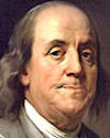
In 1752, Benjamin Franklin (1706-1790)
performed his famous (and dangerous)
electric kite experiment
which established firmly that lightning is an electrical
discharge.
Franklin himself never wrote about the story but he proofread the account which
Joseph Priestley
(1733-1804) gave 15 years after the event.
Priestley concludes that report with the comment:
"This happened in June 1752,
a month after the electricians in France had verified
the same theory, but before he heard of anything they had done."
It's unclear who those "electricians in France" are, but the following text
by Louis-Guillaume
Le Monnier appears
(in
French) in the
Encyclopédie
of Diderot and d'Alembert (71818 articles in 35 volumes, the first 28
of which were edited by Diderot himself and published between 1751 and 1766).
" A violent electric spark can modify a compass or magnetize small needles,
according to the direction given to that spark.
It has long been observed that a bolt of lightning (which is only a large electric spark)
is able to magnetize all sorts of iron and steel tools stored in boxes and to give the
nails in a ship enough magnetic properties to influence a compass at a fair distance.
This formidable fluid has simply changed into true magnets
some iron crosses of ancient belltowers
that have been exposed several times to its powerful effects. "
Indeed, many people must have wondered
why the needle of a compass goes haywire near a bolt of lightning.
However, the havoc brought about by lightning
may have precluded the proper investigation of this comparatively delicate aspect.
Domenico Romagnosi
In 1802, the Italian jurist Domenico
Romagnosi (1761-1835) experimented with a voltaic pile to charge capacitors.
He observed that their sudden discharges would deflect a nearby magnetic needle.
This raw observation was reported in newspapers. Although Romagnosi didn't
explicitly mention the connection between magnetism and electric current, at least two others
did it for him when they described his experiments:
Essai théorique et expérimental sur le Galvanisme (1804)
p. 340
by Giovanni Aldini (1762-1834).
Manuel du Galvanisme (1805)
by Joseph Izarn (1766-1847).
The crucial fact that a steady electric current does produce magnetism was finally established,
by a Danish scholar, who became famous for that:
Hans Christian Ørsted
On April 21, 1820, the Danish physicist
Hans Christian Oersted
(1777-1851) was preparing demonstrations for one of his lectures
at the University of Copenhagen.
He noticed that a compass needle was deflected when a large electrical current was
flowing in a nearby wire.
This precise instant marks the birth of
electromagnetism, the study of the interrelated
phenomena of electricity and magnetism.
Contrary to popular belief,
the discovery of Ørsted was not entirely a chance
accident (R.C. Stauffer, 1953).
As early as 1812, Ørsted had published speculations that electricity and magnetism were
connected. So, when the experimental evidence came to him, he was prepared to make the best of it.
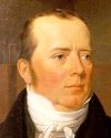
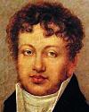
François Arago
(1786-1853; X1803) was the first person to
build an electromagnet, in September 1820, by placing iron in a wire coil.
(2008-01-04) Biot-Savart Law of Magnetostatics (1820)
The magnetic field produced by a static distribution of electric currents.
Experimentally, Ørsted
had found that a given current in a straight wire creates in its
immediate vicinity a magnetic field which seems inversely proportional
to the distance from the wire. The French physicists Jean-Baptiste Biot
and Félix Savart proposed that the
contribution of each piece of the wire actually
varies inversely as the
square of the distance to the observer. Over the entire length of the
wire, such contributions do add up to a total field which varies inversely as the
distance from the wire.
The Biot-Savart law can be precisely stated as follows:
Contribution to the Magnetostatic Field at the Origin of
a Current Element dI
at Positionr.
dB =
mor ´ dI
4p r 3
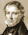
Jean-Baptiste
Biot
In this, dI is the quantity (current multiplied by the
small length it travels) which results from
integrating the current density j (current per unit of surface) over a small
element of volume.
In particular, for a thin wire circuit whose length element
ds
is traversed by a total current I (counted positively in the direction of
ds ) we have
dI = I ds.
The Biot-Savart law is for steady currents only.
For changing currents, a term that falls off as 1/r must be added,
as specified below.
Note that we're using the vector r
which goes from the location of interest to the sources.
This is a convenient viewpoint for practical computations which seek to obtain a magnetic field
at a specific point from remote distributions of current.
However, many authors
take the opposite viewpoint (opposite sign of r) to describe the
field produced at a remote location by currents located at the origin.
On October 30, 1820, the Biot-Savart law was presented to the
Académie des Sciences jointly by the physicist
Jean-Baptiste
Biot (1774-1862; X1794) and his protégé
Félix
Savart (1791-1841) who is also remembered for the logarithmic unit of musical interval
named after him (1000 savarts per decade, or about 301.03 savarts per octave).
A rounded version of the savart unit (exactly 1/301 of an octave)
was called eptaméride in an earlier scheme devised by the acoustician
Joseph Sauveur (1653-1716).
In many practical applications, the magnetic field is known to have a simple
symmetry and Ampère's Law (below) may yield the value
of the magnetic field throughout space without tedious integrations
(just like the theorem of Gauss
easily yields the electrostatic field in cases
with spherical, planar or cylindrical symmetries).
One example where no such shortcut is available is that of the
magnetic induction on the axis of a circular current loop:
In that case, all radial contributions cancel out, so the
resulting magnetic induction B is oriented along the axis
(B = Bz ).
Because of the similarity of the relevant triangles, the contribution
dBz is R/d times what's given by the
above law:
dBz = (R / d)
dB =
(R / d) ( mo I
/ 4pd2 ) ds
As the elements ds simply add up to the circumference
(2pR) we obtain:
Bz =
(R / d) ( mo I
/ 4pd2 )
(2pR)
= ½
mo I
R2 / d3
In particular, the field at the center of the loop
(d = R) is:
Bz = mo I / 2R.
Helmholtz Coil
Consider two coils (or two loops) like the above,
sharing the same vertical axis.
Let their respective altitudes be +a
and -a.
By the previous result, the magnetic induction B
(on the axis) at altitude z is:
B =
½
mo I
R2 {
[ R2 + (a-z)2 ] -3/2
+
[ R2 + (a+z)2 ] -3/2
}
The second derivative of this expression with respect to z
at z = 0 is:
B'' (0) = 3
mo I
R2 [ 4a2 - R2 ]
( R2 + a2 ) -7/2
The value a = ½ R
is thus the largest for which the magnetic induction has a
single maximum along the
vertical axis, in the center of the apparatus
(for larger values of a, B''
is positive at the center z = 0,
which indicates a minimum there).
This configuration where the separation between the two
loops is equal to their radius (2a = R)
is known as a Helmholtz coil.
It yields a magnetic induction which is
almost uniform near the center of the coil. Namely:
(2008-05-12) Magnetic Scalar Potential
(in a current-free region)
A multivalued function
whose gradient is the magnetostatic induction.
In a current-free
region of space, a scalar potential can be defined
(called the magnetic scalar potential )
whose negative gradient is the magnetostatic induction
given by the Biot-Savart law.
For a simply-connected region, such a potential is well-defined
(up to a uniform additive constant).
Otherwise, an essential ambiguity arises whenever the region contains
loops which are interlocked with loops of outside current.
In that case a continuous potential can only be defined modulo a certain
number of discrete quantities
(each of which corresponds to one interlocking outside current).
The magnetic scalar potential V for the induction
B created by a loop of thin wire is simply proportional to the
current I in that loop and to the
solid angle
W
subtended by the south side of that loop
at the location of the observer :
B
=
- grad V
V
=
-
mo I
W
4p
The solid angle
W is defined modulo
4p,
which is consistent with the aforementioned "ambiguity".
The sign convention
is such that the south side of a small loop is seen at a solid angle
which exceeds a multiple of
4p by a small positive quantity.
This is just a nice way to express the Biot-Savart law while
making it clear that, in static distributions,
all currents must circulate in closed loops
(div j = 0).
Neither this approach
nor the Biot-Savart law itself can deal with dynamic distributions
where local electric charges may vary according to the inbound flux of current.
(2008-03-10)
There are no magnetic monopoles !
(Peregrinus, 1269)
The magnetic field (magnetic inductionB)
has vanishing divergence.
It's a simple matter to establish with elementary methods
that the above Biot-Savart law
describes a field with zero divergence:
First, we can verify directly (using Cartesian expressions)
that the divergence of the Biot-Savart field vanishes at any nonzero
distance from its source dI.
We could also remark that the Biot-Savart expression
is proportional to the rotational of the vector field
dI / r.
As such, it has zero divergence.
Then, we may check that dB
has zero flux through any tiny sphere centered on
dI (this is true because of a trivial
symmetry argument).
Thus, the divergence of the Biot-Savart field is identically zero,
even at the very location of a source!
By contrast, that second part of the argument does not hold
with spheres centered on an elementary electric charge for the
Coulomb field. This is why the divergence
of the electric field turns out to be proportional to the local
density of electric charge (Gauss's Law).
The magnetic field may well have sources other than electrical currents
(including the dipole moments related to the intrinsic
spins of
point particles which are part of the modern quantum picture).
Nevertheless, all sources ever observed yield magnetic fields with no divergence.
Like all scientific facts, this can be stated as a law
which holds until disproved by experiment:
In the vocabulary of multipoles,
only monopole fields have nonzero divergence
(in particular,
any dipolar field is divergence free).
Thus, the vanishing divergence of B
is often expressed by stating that
there are no magnetic monopoles.
This was first stated in 1269 by the French scholar
Peter Peregrinus
(Pierre Pèlerin de Maricourt) who
first described magnetic poles and observed that a magnetic
pole could not be isolated (they always come in opposite pairs).
This law has survived all modern experimental tests so far and
it is postulated to remain valid in the general nonstatic case.
It is arguably the oldest of the
four equations of Maxwell.
Unfortunately, unlike the other three
(Gauss's Law,
Faraday's Law,
Ampère-Maxwell Law)
it has no universally-accepted name...
It's very often referred to as the "magnetic Gauss law",
which is rather awkward.
Calling it the "Gauss-Weber Law" would seem acceptable
because the name of Gauss is universally associated
with the electric counterpart of the law while the
magnetic flux so governed (see next paragraph)
is closely associated with the name of
Wilhelm Eduard Weber
(1804-1891) a younger colleague of Gauss after whom the SI unit of magnetic
flux (Wb) is named.
I argue that the law ought to be called Pèlerin's law
(or the Law of Peregrinus ).
The relation itself is often called
Maxwell-Thomson equation. I'm jumping on the bandwagon, although I don't
think I ever heard the term as a student.
Because of that law, the magnetic flux
(F) enclosed by a given oriented loop
is well-defined as the flux of the magnetic induction B
through any surface which is bordered
(and oriented) by that loop.
On the other hand,
two open surfaces with the same border need not have the same "electric flux"
through them, because div E isn't zero.
Searching for magnetic monopoles
A famous argument by Paul Dirac (1931)
shows that the existence of even a single true
magnetic monopole in the
Universe would imply a quantization of electric charge everywhere
(as observed).
Many physicists do not yet rule out the existence of magnetic monopoles
(like any proper physical law, Pèlerin's law
only holds until proven wrong experimentally).
A true magnetic monopole would be completely surrounded by a closed surface
traversed by a nonzero total magnetic flux.
The two ends of a thin
flux tube do
not qualify as monopoles, because the return flux
through the cross-section of the tube balances exactly the
nonzero flux traversing the rest of any closed surface
enclosing one pole (but not the other).
For example, the magnetic flux which flows
from north to southoutside a long bar magnet
is exactly balanced by the flux of the strong field which flows
from south to north inside the magnet itself.
Mathematically, we may envision an ideal flux tube
(often dubbed a Dirac string )
as the infinitely thin version of the above, namely
a line carrying, within itself, a finite
magnetic flux from one of its extremities
(the south pole) to the other (the north pole).
The total magnetic flux (F)
through a cross-section is
constant along such a Dirac string.
In the Summer of 2009, two independent teams found that actual flux tubes in
some so-called spin ices
could have cross-sections small enough to fit in the spaces between the
atoms of the crystal.
Such tubes behave like the
ideal Dirac strings presented above.
The whole thing looks as though some of the cells in the
crystal contain a magnetic monopole
while an opposite monopole is found nearby, possibly several cells away...
Those exciting discoveries do not violate
Pèlerin's law
(magnetic poles still come only in pairs, connected by
thin flux tubes).
Unfortunately, they were heralded in press releases,
review articles and popular magazines
as a "discovery of magnetic monopoles".
So, a new urban legend was born
which makes it
slightly more difficult to teach basic science...
(2008-04-25) Ampère's law:
The static version (1825)
The magnetic circulation is
mo
times the enclosed current.
André-Marie Ampère
What Gauss did in 1813 for the
Coulomb law of 1785,
André-Marie Ampère (1775-1836)
did in 1825 for the Biot-Savart law of 1820.
Unlike the law of Gauss, Ampére's law
only holds in the static case.
It had to be amended by Maxwell in 1861 for the dynamic case.
Here's Ampère's static law (1825) in differential form:
rot B = mo j
By the Kelvin-Stokes formula,
the circulation of a vector around an oriented loop is equal to the flux of
its rotational (curl) through any smooth oriented surface
bordered by that loop.
This yields Ampère's law in integral form :
mo I
º
mo
òòSj . dS
=
ò¶SB . dr
The simplest (and most fundamental) direct application of Ampère's law is
to retrieve the experimental fact which prompted the
formulation of the Biot-savart law
to begin with, namely
that the magnetic induction B due to a long straight wire
is inversely proportional to the distance from that wire:
Indeed, consider a circular loop of radius r whose axis is a
straight wire carrying a current I.
For reasons of symmetry, the magnetic induction B
on that loop is tangent to it.
Its projection on the oriented tangent is a constant B
(see sign conventions). The magnetic circulation
is 2pr B and
Ampère's law gives:
2pr B =
mo I
or, equivalently:
B =
mo I
/ 2pr
Another popular (and important) application of Ampère's law yields
the magnetic field due to an infinitely long solenoid
(of arbitrary cross-section) :
For a long solenoid consisting of n loops of wire
per unit of height (each carrying the same current I)
the magnetic induction vanishes outside and
has the following value inside the solenoid:
B = mo n I
This can be established by noticing first
that the direction
of the magnetic induction B must be everywhere vertical
(i.e., parallel to the
axis of a solenoid with horizontal cross-section).
That is so because the horizontal contribution of each element of current is
exactly canceled by the horizontal contribution from its mirror image with respect
to the horizontal plane of the observer.
We may then apply
Ampère's law to any rectangular loop with two vertical sides
and two horizontal ones (on which the circulation of B is zero,
because it's perpendicular to the line element).
This establishes that the magnetic field is constant inside the solenoid and constant outside
of it, with the difference between the two equal to the value advertised above.
(The fact that the constant value of the induction outside of the solenoid must be zero is
just common sense, or else the magnetic energy of the solenoid
per unit of height would be infinite.)
Sneak Preview :
In 1861, Maxwell was able to amend the static law of Ampère
into the following generalization, which holds in all cases
(including changing charge distributions).
Ampère-Maxwell Law (1861)
rot B-
1
¶E
= mo j
c2
¶t
We shall postpone the
discussion of this crowning achievement
(which made the entire structure of electromagnetism consistent)
so we can present first a key breakthrough
made by Faraday on August 29, 1831
(when James Clerk Maxwell was 2 months old):
The law of magnetic induction.
(2005-07-19) Faraday's Law of Electromagnetic Induction
(1831)
On the electric circulation induced around
a varying magnetic flux.
Michael Faraday
Michael
Faraday (1791-1867) was the son of a blacksmith,
and a bookbinder by trade.
Effectively, he would remain mathematically illiterate,
but he became an exceptionally brilliant experimental scientist who would lay
the conceptual foundations that occupied
several generations of mathematical minds.
In 1810, Faraday started attending the lectures that
Humphry Davy (1778-1829) had been giving at
the Royal Institution of London since 1801.
Humphry Davy
John Fuller
In December 1811, Faraday became an assistant of Davy,
whom he would eventually surpass in knowledge and influence.
Faraday was elected to the Royal Society in 1824,
in spite of the jealous opposition of Sir Humphry
Davy (who was its president from 1820 to 1827).
In February 1833,
Faraday became the first Fullerian Professor of Chemistry
at the Royal Institution The chair was endowed by his mentor and supporter
John "Mad Jack" Fuller
(1757-1834).
Arguably, the greatest of Faraday's many scientific contributions was
the Law of Induction which he formulated in 1831.
After explaining the 1820 observation of
Ørsted in terms of what
we now call the magnetic field,
Faraday did much more than invent
the electric motor.
Eventually, he opened entirely new vistas for physics.
He proposed that light itself was an electromagnetic
phenomenon and lived to be proven right mathematically by his young friend,
James Clerk Maxwell.
Faraday's Law (1831)
rot E +
¶B
= 0
¶ t
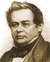
Heinrich Lenz
Heinrich Friedrich "Emil Khristianovich"
Lenz (1804-1865). Lenz's Law (1833).
The magnetic flux...
F = B . S
dF =
dB . S +
B . dS
First term = Magnetic Induction. Second Term = Lorentz Force.
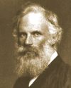
(2008-04-02) Self-Inductance (Henry, 1832)
On the electric induction produced in a circuit by its own magnetic field.
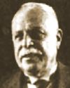
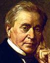
Joseph Henry, 1875
The American physicist Joseph Henry (1797-1878)
discovered the law of induction independently of
Faraday. Henry went on to remark that the magnetic field created by a changing
current in any circuit induces in that circuit itself an
electromotive force which tends to oppose the change in current.
(2008-04-30) Ampère's law
generalized by Maxwell (1861)
The Ampère-Maxwell law holds even with changing charge distributions.
A simple way to show that the above static version of
Ampère's law
fails in the presence of changing electric fields is to consider how a
capacitor
breaks the flux of current it receives from a conducting wire:
An open flat surface between the capacitor's two plates
has no current flowing through it, unlike a surface
with the same border which the wire happens to penetrate.
In 1861, Maxwell realized that, since electric charge is conserved,
a difference in the flux of current
through two surfaces sharing the same border must imply a change
in the total electric charge q
contained in the volume between those two surfaces.
By Gauss's theorem, this translates into
a changing flux of the electric field through
the closed surface formed by the two aforementioned open surfaces.
More precisely, and remarkably, the "missing" flux of the current density
j is exactly balanced by the flux of the vector
eo ¶E/¶t.
Maxwell identified this as the density of a quantity
he called displacement current.
He saw that the sum of the actual current and the displacement
current was divergence-free.
This made that sum a prime candidate
for taking on the role played by the ordinary density of current in
the static version of Ampère's law.
Therefore,
Maxwell proposed that Ampère's law
should be amended accordingly:
rot B = mo
( j + eo ¶E/¶t )
Putting the fields on one side and the sources on the the other, we obtain:
Ampère-Maxwell Law (1861)
rot B-
1
¶E
= mo j
c2
¶t
At this point, we merely
define c as a convenient constant satisfying:
eo
mo c 2
= 1
The paramount fact that c turns out to be the
speed of light will be seen to be a
consequence of putting all of Maxwell's equations together...
(2005-07-18) On the History of Maxwell's Equations
The 4 basic laws of electricity and magnetism, discovered one by one.
Gauss's Magnetic Law = Maxwell-Thomson equation = Pélerin's Law (1269).
Gauss' Electric Law = Coulomb's Law = Poisson's equation.
Faraday's Law of Induction.
Ampère's Law (became Maxwell-Ampère equation).
(2005-07-09) Maxwell's Equations Unify
Electricity and Magnetism
They predicted electromagnetic waves before Hertz demonstrated them.
I have also a paper afloat, with an electromagnetic theory of light, which,
till I am convinced to the contrary, I hold to be great guns.
James Clerk Maxwell (1831-1879)
[ letter to
Charles H.
Cay (1841-1869) dated January 5, 1865 ]
Maxwell's equations govern the electromagnetic
quantities defined above:
The electric fieldE
(in V/m or N/C).
The magnetic inductionB
(in teslas; T or Wb/m 2).
The density of electric charge r
(in C/m3 )
The density of electric currentj
(in A/m2 )
Maxwell's Equations (1864)
in modern vectorial form :
rot E +
¶B
= 0
div E =
r
¶ t
eo
rot B-
1
¶E
= mo j
div B = 0
c2
¶t
The three electromagnetic constants involved are tied by one equation:
eo mo c 2
= 1
eo
is the electric permittivity of the vacuum
(in F/m)
(2005-07-09)
Continuity Equation & Franklin-Watson Law (1746)
The continuity equation
expresses the conservation of electric charge.
A direct consequence of Maxwell's equations is the following relation,
which expresses the conservation of electric charge
(HINT: div rot Bvanishes).
This conclusion holds if and only if the 3 aforementioned
electromagnetic constants are related as advertised above.
Continuity Equation
div j +
¶r
= 0
¶t
Benjamin Franklin
Historically, the relation is reversed:
The conservation of electric charge
had been formulated before 1746, independently by
Benjamin Franklin (1706-1790) and
William
Watson (1715-1787).
This was more than a century before Maxwell used it to
generalize Ampère's law
into the proper equation which made the whole theoretical structure perfect.
(2005-07-09)
Electromagnetic Radiation :
From light to radio waves.
Electromagnetic fields propagate at the speed of light (c).
Using the identityrot rot V = grad div V - DV
when r = 0 and
j = 0,
Maxwell's equations imply that
any electromagnetic component y
verifies:
1
¶ 2 y
= Dy
c 2
¶ t 2
This wave equation shows that
electromagnetism propagates at celerity c in a vacuum.
Thus, Maxwell's equations support the electromagnetic theory of light
which
Michael Faraday
had proposed well before all the evidence was in.
(He engaged in such speculations in 1846, at the end of one of his famous lectures
at the Royal Institution, because he had run out of things to say that particular Friday night!)
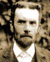
George Francis FitzGerald
In 1883, the Irish physicist
George FitzGerald (1851-1901)
remarked that an oscillating current ought to generate
electromagnetic radiation (radio waves).
FitzGerald is also
remembered for his 1889 hypothesis that all moving objects are
foreshortened in the direction of motion
(the relativisticFitzGerald-Lorentz contraction).
The propagation of radio waves was first
demonstrated experimentally in 1888, by Heinrich Rudolf
Hertz (1857-1894).
(2005-07-15)
Electromagnetic Energy & Poynting Vector
The Lorentz force transfers energy between the
field and the charges.
The power F.v of the Lorentz force is
q E.v. Thus, the power received by the electric charges per unit of
volume is E.j.
The charge carriers may then convert the power so received from the local electromagnetic
field into other forms of energy (including the kinetic energy of particles).
Conversely, E.j can be negative, in which case there is
a transfer of energy from the charge carriers to the field.
One process can be seen as a time-reversal of the other.
In this, it is essential to retain both the
retarded and advanced solutions of Maxwell's equations;
the motion of the sources and the changes in the field
may cause each other !
The quantity E.j may be expressed in terms of the electromagnetic
fields by dotting into
- E/mo
both sides of the Ampère-Maxwell equation:
Plugging that into the previous equation, we obtain an important relation:
Electromagnetic Balance of Energy Density :
Poynting Theorem (1884)
div (
E ´ B
) +
(
eoE 2
+ B 2/ mo
) =
- E . j
mo
¶t
2
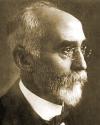
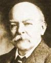
John Henry Poynting
This is due to a pupil of Maxwell,
John
Henry Poynting (1852-1914).
S = E´B / mo is the Poynting vector.
In the above, the right-hand side is the opposite
of the power delivered by the field to the sources, per unit of volume.
So, it's the density of the power released by the sources to the field.
The left-hand side is thus consistent with the following
energy for the electromagnetic field:
Electromagnetic Energy Density
1/2 eo
( E 2 +
c2 B 2 )
The above Poynting theorem states that, the variation of this
energy in a given volume comes from power that is either delivered directly by inside sources
or radiated through the surface, as the flux of the Poynting vector.
In the context of
Classical Field Theory,
the above is the Hamiltonian density, whereas
the Lagrangian density of the electromagnetic
field is a Lorentz scalar
(a mere pseudo-scalar like
E.B won't do) namely:
Lagrangian Density
1/2 eo
( E 2 -
c2 B 2 )
Identifying the above with the usual formulas for the Hamiltonian
(H=T+U) and the Lagrangian (L=T-U)
we may think of the square of E
as a kinetic term (T) and the square of B
as a potential term (U).
The analogy is more compelling when a special
gauge is used which makes the electrostatic
potential (f) vanish everywhere,
as is the case for the standard
Lorenz gauge in the particular case of
a crystal of magnetic dipoles.
For in such cases, the electric field consists entirely of
time-derivatives of A...
The above is for the electromagnetic field by itself.
In the presence of charges which interact with the field in the
form of a density of Lorentz forces, the corresponding Lagrangian density
of interaction should be added:
Lagrangian Density
1/2 eo
( E 2 -
c2 B 2 )
-
( r f - j.A )
Still missing are all the non-electromagnetic terms needed to determine correct expressions
of the conjugate momenta and Hamiltonian density...
(2005-07-15)
Electromagnetic Planar Waves (Progressive Waves)
The simplest solutions to Maxwell's equations,
away from all sources.
In the absence of electromagnetic sources
( r = 0, j = 0 ) we may look for
electromagnetic fields whose values do not depend
on the y and z cartesian coordinates.
A solution of this type is called a
progressive planar wave and it may be established
directly from the aboveequations of Maxwell,
without invoking the electromagnetic
potentials introduced below.
Indeed, when all derivatives with respect to y or z vanish,
the 8 scalar relations which express Maxwell's equations
in cartesian coordinates become:
¶ Bx
=
0
¶ Ex
=
0
¶ x
¶ x
0
=
1
¶ Ex
0
=
-
¶ Bx
c 2
¶ t
¶ t
-
¶ Bz
=
1
¶ Ey
-
¶ Ez
=
-
¶ By
¶ x
c 2
¶ t
¶ x
¶ t
¶ By
=
1
¶ Ez
¶ Ey
=
-
¶ Bz
¶ x
c 2
¶ t
¶ x
¶ t
To solve this, we introduce the new variables
u = t - x/c
and v = t + x/c
For any quantity y,
the two expressions of the
differential form dy
yield the expressions of the partial derivatives with respect to the new variables :
dy =
¶ y
dt +
¶ y
dx =
¶ y
du +
¶ y
dv
¶ t
¶ x
¶ u
¶ v
dt = 1/2 ( dv + du )
and
dx = c/2 ( dv - du )
Therefore,
ì ï í ï î
¶ y
=
1
(
¶ y
- c
¶ y
)
¶ u
2
¶ t
¶ x
¶ y
=
1
(
¶ y
+ c
¶ y
)
¶ v
2
¶ t
¶ x
We may apply this back and forth when y is one of
the cartesian components of E
or B, using the above relations between those.
For example:
¶ Ey
=
1
¶ Ey
-
c
¶ Ey
= -
c2
¶ Bz
+
c
¶ Bz
= c
¶ Bz
¶ u
2
¶ t
2
¶ x
2
¶ x
2
¶ t
¶ u
Thus,
Ey - c Bz
doesn't depend on u.
Likewise, neither does
Ez + c By
Similarly, both
Ey + c Bz
and
Ez - c By
do not depend on v.
In 1871, Maxwell himself predicted this as a consequence of
his own equations.
In 1876,
Adolfo Bartoli (1851-1896)
remarked that the existence of radiation pressure is also an unavoidable consequence
of thermodynamics.
(Radiation pressure is thus sometimes called Maxwell-Bartoli pressure.)
Maxwell-Bartoli pressure was first demonstrated experimentally by
Pyotr Lebedev in 1899.
In 1873,
Sir William Crookes (1832-1919)
believed that he had demonstrated radiation pressure when he came up with
the so-called
radiometer (or
light-mill) displayed
on his coat-of-arms.
This ain't so, despite what many sources still state. Radiation pressure is too weak to
turn the vanes of such a radiometer and its theoretical torque
opposes the observed rotation!
(The dark sides of the vanes are actually receding.)
Crookes' radiometer is actually a subtle heat engine in which the
rarefied gas in the glass enclosure plays an essential rôle
(it wouldn't work in a hard vacuum).
The moving torque is due to what's called the "thermal creep" of the gas molecules
near the edges of the vanes, where a substantial temperature gradient is maintained...
This was first correctly explained by
Osborne Reynolds (1842-1912)
in a paper which
Maxwell refereed the year he died (1879).
Maxwell published immediately his own paper on the subject, giving credit to Reynolds for the
key idea but criticizing his mathematics
(the Reynolds paper itself was only published in 1881).
Pyotr Lebedev
The first proper measurement of radiation pressure
was made in 1899 by
Pyotr Lebedev (1866-1912).
In 1901, the pressure of light was measured
at Dartmouth by
Nichols and
Hull
to an accuracy of about 0.6% (the original
Nichols radiometer
is at the Smithsonian).
To avoid the aforementioned effect (dominant in
Crookes radiometers)
a Nichols radiometer must operate in a high vacuum.
(2005-07-13)
Electromagnetic Potentials & Lorenz Gauge
Devised by Ludwig Lorenz in 1867
[when H.A. Lorentz was only 14].
Since Maxwell's equations assert that
the divergence of B vanishes,
there is necessarily a vector potentialA
of which B is the rotational (or curl).
B = rot A
Faraday's law now reads rot [ E +
¶A/¶t ] = 0 .
The square bracket is the gradient of a scalar potential, called
-f for consistency with electrostatics:
E =
- grad
f - ¶A/¶t
These two equations do not uniquely determine the potentials,
as the same fields are obtained with the following substitutions of the
potentials, valid for any
smooth scalar field y.
A ¬ A
+ grad y
f
¬ f
-
¶y/¶t
This leeway can be used to make sure the following equation is satisfied,
as proposed by Ludwig Lorenz in 1867.
(Watch the spelling... There's no "t".)
The Lorenz Gauge (1867)
div A +
1
¶f
= 0
c2
¶t
The Lorenz Gauge doesn't eliminate the above type of leeway.
It restricts it to a free field y
propagating at celerity c, according to the wave equation :
Dy -
1
¶ 2 y
= 0
c 2
¶ t 2
The two Maxwell equations which don't involve electromagnetic sources are equivalent to the
above definitions of E and B in terms of
electromagnetic potentials.
Using the Lorenz Gauge, the other two equations reduce to the following relations
between the electromagnetic sources and the potentials:
D'Alembert's Equations
Df
-
1
¶f
=
r
c2
¶t
eo
DA
-
1
¶A
= -mo j
c2
¶t
Without the Lorenz Gauge, more complicated relations would hold:
Df
-
1
¶f
=
r
( div A +
1
¶f
)
c2
¶t
eo
¶t
c2
¶t
DA
-
1
¶A
=
-mo j + grad
( div A +
1
¶f
)
c2
¶t
c2
¶t
Formerly viewed as a mere mathematical convenience
(which Maxwell himself didn't like at all)
the Lorenz gauge is now considered fundamental,
because quantum theory assigns a physical
significance to the potentials.
In the
Aharonov-Bohm effect (1959)
interference patterns produced by charged particles travelling outside of a solenoid are seen to depend
on the value of a steady current through the solenoid,
although the electromagnetic fields outside of the solenoid do not depend on it...
The Lorenz gauge is relativistically covariant
(if it's true in one frame of reference it's true in all of them).
This isn't the case for other popular gauges, including the
Coulomb gauge (div A = 0)
once favored by Maxwell.
Such putative gauges are thus incompatible with the
objectivity of potentials.
The expressions of the Lagrangian, Hamiltonian and canonical momentum
of a charged particle in an electromagnetic field do depend explicitly on the potentials,
although the classicalLorentz force derived from them does not
depend on the choice of a gauge
(see elsewhere on this site for a proof).
Canonical momentum of a particle of mass m, charge
qand velocityv
(2005-07-15)
Retarded and advanced potentials (& free photons)
General solutions of Maxwell's equations
using the Lorenz gauge.
As shown above, the miraculous effect of
the Lorenz gauge is that
it effectively decouples electricity and magnetism
to turn Maxwell equations into parallel
differential equations that can formally be solved using standard techniques
(the d'Alembert equations are named after
Jean-le-Rond d'Alembert,
who solved the related homogeneous wave equation).
One relation equates second derivatives of the electric potential
f
to the electric density
r.
The other [vectorial] relation
equates the same derivatives of each component of
the vector potential A to the corresponding component of
the density of current j.
The mathematical solution for each component (and, therefore,
for the whole thing)
can be expressed as the sum of three terms said to be, respectively,
retarded, advanced and free :
f = (1- a)
f-
+ a f+
+ fo A = (1- a)
A-
+ a A+
+ Ao
Usually, only a = 0
is considered, for the causality reasons
discussed below.
a = 1 is
an alternate choice which reverses the arrow of time. In 1945,
Wheeler
& Feynman fantasized about the possibility of
a = ½.
The free terms (superscripted o ) are exactly what we have
already encountered
as the remaining degrees of freedom after imposing
the Lorenz gauge. They correspond mathematically to
solutions of the homogeneous differential equations
(zero charges and currents characterize free space).
Happily, the fact that they appear again here means that the choice of that
gauge really involved no loss of generality.
(This is not coincidental but we may pretend it is.)
The retarded terms are given by the following
expressions, proposed by
Alfred-Marie
Liénard (1869-1958; X1887) in 1898
and by
Emil Wiechert (1861-1928)
in 1900. They're known as the
Liénard-Wiechert potentials.
Electrodynamic Retarded PotentialsA-and f-
f-(t,r)
=
òòò
r( t - ||r-s|| / c , s )
d3s
4peo
|| r - s ||
A-(t,r)
=
òòò
mo j ( t - ||r-s|| / c , s )
d3s
4p
|| r - s ||
This is similar to the expressions obtained in the static cases
(electrostatics, magnetostatics) except
that the fields we observe here and now
depend on a prior state of the sources.
The influence of the sources is delayed by the time it takes
for the "news" of their motions to be broadcasted at speed c.
The so-called advanced potentials
( A+ and f+ )
are formally obtained by making c negative
in the above retarded expressions
(or equivalently by reversing the
arrow of time).
This is just like what we've already encountered
in the case of planar waves,
with two possible directions of travel.
However, the physical interpretation is not nearly as easy now that we're
dealing with some causality relationship between the field and its
"sources".
Advanced potentials make the situation here and now
(potentials and/or fields) depend on the future
state of remote "sources".
Such a thing may be summarily dismissed as "unphysical" but this fails
to make the issue go away.
Indeed, quantum treatments of electromagnetic fields (photons in
Quantum Field Theory )
imply that a field can create some of its sources in the form of charged
particle-antiparticle pairs.
What seems to be lacking is the coherence
of such creations because of statistical and/or thermodynamical
considerations (which feature a pronounced arrow of time).
I don't understand this. Nobody does...
What's clear, however, is that the distinction between past and future vanishes
in stationary cases.
This makes advanced potentials relevant and/or necessary,
without the need for mind-boggling philosophical considerations.
We've only shown
(admittedly skipping the mathematical details)
that potentials that obey the
Lorenz gauge would necessarily be given by the
above formulas (possibly adding advanced
and free components).
Conversely, we ought to determine now what restrictions, if any,
(pertaining to the sources r and j)
would make the above solutions verify the assumed Lorenz gauge.
However, we shall postpone this discussion
to present first a clarification of the physics...
(2005-08-21)
Electrodynamic Fields Caused by Moving Sources
An expression derived from the
Liénard-Wiechert retarded potentials.
Let
r and j denote
r ( t - R / c
, s ) and
j ( t - R / c , s ).
As always, R =
|| r - s ||
is the distance from a source (located at s)
to the observer (at r).
The following expressions of the fields then hold:
Electrodynamic fields obtained from retarded potentials :
E(t,r)
=
1
òòò
[
r
( r - s )
+
( ¶ r / ¶t )
( r - s )
-
¶ j /
¶t
] d3s
4peo
R 3
cR 2
c 2 R
B(t,r)
=
mo
òòò
[
j ´
( r - s )
+
( ¶ j /
¶t ) ´
( r - s )
] d3s
4p
R 3
cR 2
In the static case, only the first term of either expression subsists
and we retrieve either the Coulomb law
of electrostatics or the Biot-Savart law
of magnetostatics.
A changing distribution of charges and currents generates the additional
terms whose amplitudes dominate at large distances
because they only decrease as 1/R.
This is what makes radio transmission practical!
On 2009-09-06,
Henryk Zajdel
wrote: [edited summary]
I just stumbled on your website. It is brilliant !
However, [the above formulas] do not look right to me.
Could you direct me to a publication where they are derived?
I find those expressions for the electromagnetic fields
caused by dynamic sources very enlightening.
Personally, I discovered them after
establishing the dipolar
solutions of Maxwell's equations, which strongly suggest such formulas.
They are now known as
Jefimenko's equations,
in honor of
Oleg D. Jefimenko (1922-2009).
They were probably discovered privately many times.
According to Kirk T. McDonald (1997)
the first textbook which mentions them is the second edition
of Panofsky and Phillips (1962).
Here's an outline of how those formulas can be derived from the well-known
integrals giving the retarded potentials.
In either of those integrals, t
is a constant and so are the coordinates x,y,z of r.
Differentiation with respect to x,y,z or t is thus performed by
differentiating the integrand,
which involves only numerical expressions of the
following type (using the notations introduced at the outset):
k(R) f ( t-R/c , s )
In this, k(R) is simply proportional to 1/R
(but we may treat it like some unspecified function of R ).
Both factors depend on x,y,z only because R does.
The function f depends on time; k doesn't.
The chain rule yields:
¶ f
=
¶ f
( t -
R
)
= -
1
¶ R
¶ f
¶ x
¶ t
¶ x
c
c
¶ x
¶ t
¶ R / ¶ x
is obtained by differentiating R2 =
(r-s)2 . Namely:
R dR =
( x-sx ) dx +
( y-sy ) dy +
( z-sz ) dz
¶ f
= -
x - sx
¶ f
¶ x
c R
¶ t
From this basic relation, and its counterparts along y and z, we obtain:
- gradf
=
¶ f
r - s
¶ t
c R
The same relations applied to the components
fx fy fz
of a vector F yield:
rotF
=
¶ F
´
r - s
¶ t
c R
Another relation
(needed only in the next section)
involves a dot product :
div F
= -
¶ F
·
r - s
¶ t
c R
Handling the scaling part introduced above as k(R) is similar
but less tricky conceptually, because k is simply a
scalar function of a single argument (the distance R
between source and observer) with a straight derivative
k'. (As k is proportional to 1/R,
we have k'(R) = -k/R.)
The conclusion follows from two general identities of
vector calculus and one
trivial equation (expressing that k is time-independent) namely:
rot (k F) =
grad k ´ F
+
k rot F
- grad (k f )
=
-
fgrad k
-
k gradf
- ¶/¶t (k F)
=
- k
¶F/¶t
The first line yields the expression of B,
the sum of the last two gives E.
(2010-12-06)
Electrodynamic Fields Causing Sources to Move
An expression derived from the
Liénard-Wiechert advanced potentials.
Let's now forget the aura of mystery traditionally associated with
advanced solutions.
Reversing the direction of time simply reverses causality.
Bluntly, when the photons kick the electrons,
the values of the fields are related to the values of the
so-called "sources" at a later time (the sources
are not the causes in this case; their name is misleading).
Now,
r and j denote
r ( t + R / c
, s ) and
j ( t + R / c , s ).
Electrodynamic fields obtained from advanced potentials :
E(t,r)
=
1
òòò
[
r
( r - s )
-
( ¶ r / ¶t )
( r - s )
-
¶ j /
¶t
] d3s
4peo
R 3
cR 2
c 2 R
B(t,r)
=
mo
òòò
[
j ´
( r - s )
-
( ¶ j /
¶t ) ´
( r - s )
] d3s
4p
R 3
cR 2
Compare this formally to the
similar expressions
for retarded potential and notice the changes
of sign that occur in the second column but not the third!
Thoses changes can be traced down to the beginning of the proof outlined above
for retarded potentials, since for a function
f ( t+R/c , s ) :
¶ f
=
¶ f
( t +
R
)
= +
1
¶ R
¶ f
¶ x
¶ t
¶ x
c
c
¶ x
¶ t
The corresponding change of sign (compared to retarded potentials)
applies to the dynamical parts of
grad f or
rot A but does not formally affect
the ¶A/¶t
component of E.
One important consequence of such changes of signs is that it affects the
distant fields in a way which reverses
the sign of Larmor's formula.
In other words, contrary to popular belief, an accelerated or decelerated
charge need not radiate electromagnetic energy away.
It does so only when the change of its motion is the cause of changing
fields, not when it's the result of such changing fields.
Electromagnetic energy always flows from cause to effect.
(2005-08-11)
Radiated Energy (Larmor Formula, 1897)
Accelerated [bound] charges radiate energy away, or do they?
Consider the dipolar solutions to Maxwell's
equation (retarded spherical waves) presented
elsewhere on this site.
At a large distance, the dominant field components are proportional
to the second derivatives p'' or m''.
For an electric dipole, the dominant
far-field component of the Poynting vector
( E´B / mo )
is thus in the radial direction of the normed vector u:
mo
( u ´
d2 p
)
2
u
(4p r)2 c
dt 2
This is a radial vector whose length is proportional to
sin2 q =
1 - cos2 q
(where q is the angle between
p'' and the direction of u).
Its flux through the surface of the sphere of radius r is the
total power radiated away:
mo
(
d2 p
)
2
ò
p
(1 - cos2 q )
(2p r 2
sin q )
dq =
mo
|| p''|| 2
(4p r)2 c
dt 2
0
6p c
Likewise, the total power radiated by a magnetic dipole is :
( mo / 6p c3 )
|| m''|| 2
Let's use a subterfuge
to compute the power radiated away by a single charge q
near the origin: Place a charge -q (a "witness") at the origin itself.
At large distances, the resulting variable dipole
p = q r(t)
would produce essentially the same dynamic field
(at time t+r/c)
as the lone moving charge q (as long as its acceleration does not vanish
and its distance to the origin remains small).
This translates into the following so-called
Larmor formula (derived in 1897 by
Joseph Larmor, 1857-1942):
Power radiated by a charge q
mo q 2
(
d2 r
)
2
6p c
dt 2
Note that the above was obtained from field expressions based on
retarded potentials which are appropriate when
changing sources cause changing fields.
If that causality relationship is reversed, the
fields based on advanced potentials
should be used instead. They yield a formula whose sign is the
opposite of the above (which would indicate that an accelerated or
decelerated charge receives energy).
In other words, energy always flows from the cause to the effect.
The above argument skirts near-field difficulties, but it seems inadequate whenever
the moving charge is not confined to the immediate vicinity of
the artificial "witness" charge.
In particular, we don't obtain a clear picture of what happens,
in the long run, when a charge is subjected to
a constant acceleration...
It has been argued that no power would be lost away in this case,
which (according to General Relativity) is equivalent to a motionless charge
in a constant gravitational field.
Even so, a varying gravity ought to make charges radiate
(classically, at least).
A promising way out of that dilemma (2006-10-16)
is to consider the thermal nature of the above exchange of energy,
allowing the formula to hold, in some statistical way, as the classical counterpart
of a quantum effect...
Indeed, in 1976, W.G. Unruh found
that an acceleration g (or, equivalently, a gravitational field)
entails a heat bath whose temperature T
is proportional to it :
(2005-08-09)
The Lorentz-Dirac Equation
Classical Theory of the Electron. Strange inertia of charged particles.
The motion of an electron (point particle of charge q) submitted to a force
F has been described in terms of the following 4-dimensional equation,
where (primed) derivatives of the position R are with
respect to the particle's proper time
t [ defined via:
(c dt)2 = (c dt)2-(dx)2-(dy)2-(dz)2 ].
Lorentz-Dirac Equation (1938)
m R'' = F +
mo q 2
[ R''' +
| R' ><R' |
R''' ]
6pc
c2
The Abraham-Lorentz equation is the non-relativistic
version of this (using "absolute" time and
retaining only the first term of the bracket).
| R' ><R' | is a square tensor
(the product of the 4D velocity and its dual).
The bracketed sum is only relevant for a point particle of nonzero charge.
Its nature has been highly controversial since 1892, when
H.A. Lorentz
first proposed a
Theory of the Electron derived microscopically from
Maxwell's equations and from
the expression of the electromagnetic force now named after him.
Lorentz would only consider the electromagnetic part of the
rest mass m (i.e., 3m/4).
In 1938, Paul Dirac derived the above covariantly,
for the total mass m.
Physically, the initial value of the acceleration (R'' )
in this third-order equation cannot be freely chosen
(so the overall constraints are comparable to those of an ordinary newtonian equation).
Almost all mathematical solutions are unphysical ones,
which are dubbed
self-accelerating or runaway because they would make
the particle's energy grow indefinitely, even if no force was applied.
However,
more than one initial value of the acceleration could make physical
sense. The wholly classical Lorentz-Dirac equation
thus allows a nondeterministic behavior more often associated with
quantum mechanics.
The Lorentz-Dirac equation has other weird features, including the need
for a so-called preacceleration contradicting causality,
since the equation would require an electron to anticipate any impending pulse of force...