2015
International Year of Light and Light-Based Technologies
Geometrical Optics : Rays and Shadows
(2010-11-25)
Radius of curvature of a concave mirror...
Curvature of a mirror magnifying k=3 times an object d=22 cm away?
Mirrors were the first optical systems to be analyzed mathematically...
That's a good opportunity to practice elementary geometry.
For this exercise, we shall only need two optical principles:
Rays from an object point emerge as if they came from its image.
On a mirror, the angle of incidence is equal to the angle of reflection
(Hero of Alexandria, first century AD).
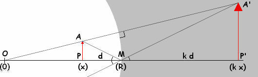
Let's choose a coordinate system where the origin O is the center of curvature of the mirror.
The mirror intersects the x-axis at a point M,
whose abscissa R is the radius of curvature which we're seeking.
Consider an object A of small height
above the point P on the axis;
both points are at abscissa x.
Let A' be the (virtual) image of A,
above a point on the axis which we'll call P' .
If we're told that our object is magnified by a factor k = 3 ,
we know that P'A' is k times PA.
Any ray going through the center O of the sphere is reflected back onto itself,
so OA and OA' are collinear (O, A and A' are aligned).
Therefore, the triangles OPA and OP'A'
are similar.
So, by the theorem of Thales,
OA' is to OA what A'P' is to AP.
Both ratios are equal to k.
This is to say that the abscissa of A' or P' is k x.
On the other hand,
consider the ray from A which is reflected at the point M of the
mirror on the x-axis, at abscissa R.
Because the angle of incidence (the inclination of MA)
is equal to the angle of reflection (the inclination of MA' )
we have, again, two similar triangles (MPA and MP'A' )
in a ratio k. So, MP' is equal to k
times the distance d
which we are given (as the distance of 22 cm
from the mirror to the object).
This shows that the abscissa of A'
(or P' ) is equal to R+kd. Therefore:
R + kd = k x = k (R-d)
Solving this for R, we obtain R = 2 d / (1-1/k) = 66 cm.
Focal Length of a Concave Mirror :
Importantly, the above can be forcibly recast into a standard form:
1
=
1
+
1
f
p
p'
Using the following equivalences:
p = x (distance from the optical center to the real object).
p' = k x (distance from O to the image).
f = R/2 (a positive quantity for a
concave mirror).
This last equation can be construed as the definition of the focal length
of a concave mirror, which is thus shown to obey an
optical equation similar to what's established for a thin-lens in the
next section.
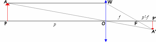
(2015-06-29) Thin-Lens Equation. Definition of the focal length.
Relation between the positions p and p' of an object and its image.
A thin-lens
is an ideal system which can be approximated by an axial-symmetric
thin piece of glass bounded by two polished spherical surfaces.
I use an hyphen to denote the "thin-lens"
optical concept, as opposed to an actual lens that
happens to be a good approximation of such a thing because it's not too thick...
Actually, the best thin-lenses have a substantial
thickness to them (crystal balls are a striking example).
What really qualifies an optical system as a thin-lens is the existence of an
optical center, as defined next.
Unfortunately, this hyphenated clarification is not universally adopted
(in fact, at this writing, I seem to be the only one advocating it).
Two physical properties of a thin-lens are sufficient to establish
its ability to form real images of real objects near the optical axis, namely:
The center O of the lens is an optical center
(i.e., rays through it are not deflected). That's very nearly true
for rays which have low inclination with respect to the optical axis if
the thickness of the glass at the center is small
(hence the qualifier thin).
Anyincident ray parallel to the optical axis emerges as a ray
emanating from the image focal point F.
The distance OF is a characteristic ( f ) of the lens called its
focal length.
(We'll see later that the value of f can be obtained
from the lens-maker formula.)
Optical diagrams are intended to portrait the situation near the optical axis but
exaggerated radial distances are used for clarity.
The usual convention is to make the optical axis horizontal, with light shining
from left to right.
A converging thin-lens is represented by a vertical line
with two outward-pointing arrows (they would be inward-pointing for a diverging lens).
Objects and images (usually, only one of each) are vertical arrows
originating on the horizontal optical axis.
Here, we consider an object A above a point P on the axis,
at distance p from the optical center O.
Its image A' is located below a point P'
on the axis, at a distance p' from O.
The point W is where a ray from A parallel to the optical axis
meets the central plane of our lens.
The heights of the similar triangles APO (or OWA) and A'P'O
are proportional to p and
p'. With this in mind, we apply the
theorem of Thales again
to the triangles FOW and FP'A' and obtain this relation:
f / p = ( p'- f ) / p'
It boils down to the following celebrated relation between p and p' :
The Thin-Lens Equation :
1
=
1
+
1
f
p
p'
We only derived that formula in the case of a converging lens
(positive focal length) real object (positive p) and
real image (positive p' ).
However, it remains valid in all other cases, with the following sign conventions:
For a divergent lens, the focal length f is negative.
For a virtual object, p is negative.
For a virtual image, p' is negative.
The use of concave lenses (negative focal length)
to relieve myopia was first advocated by
Nicholas of Cusa (1401-1464).
(2018-01-04) Focusing distance and working distance :
Both differ from the aforementioned optical positions ( p or p' ).
The focusing distance D is the distance between an object and its image.
When a distance scale is provided on a commercial lens,
this is the intented meaning. On commercial cameras, the location
of the focal plane is often discreetly engraved so that the focusing distance
can be directly measured with a tape-measure.
In the case of a thin-lens, the focusing distance D
is simply the sum of the object and image positions :
D = p + p'
Working Distance :
In macro-photography, the working distance is what
separates an object in sharp focus (on the optical axis) from the
front surface of the lens.
The least such separation is the minimum working distance (MWD)
which is sometimes advertised instead of the closest focusing distance
for commercial lenses.
This can be very small;
it would even be negative for a lens
which could bring into focus virtual objects within itself
(a virtual object is where the rays of a convergent incident beam meet).
(2015-07-01)
Hyperfocal Distance
Position of the nearest in-focus objects when the lens is set to infinity.
It's convenient to define the position of an object as the
parameter p which appears in the
thin-lens equation (or its counterpart for more general
optical systems, analyzed later).
This is only indirectly related to the distance
used by photographers
(the actual distance between the film/sensor and the object, which may or
may not be in sharp focus).
The distinction is made between objects in sharp focus
(whose images are precisely located on the sensor)
and other in-focus objects which project a pencil
of light thats intersects the plane of the sensor on a
spot whose diameter does not exceed the diameter
of the accepted circle of confusion.
In traditional 35 mm photography,
the diameter of the circle of confusion is commonly taken to be 0.03 mm.
For crop-sensor cameras (with a crop factor around 1.5)
that would be equivalent to 0.02 mm, which corresponds to the width of
about 5 pixels in the Nikon D5500 DSLR.
It's just a single pixel in an image resized to 1200 by 800 pixels.
(2010-11-26)
Paraxial Optics. Ray Transfer Matrix (RTM).
Each optical component acts on the distance and inclination of a ray.
Elementary geometry is great in simple cases but fails to give the rules by
which complicated optical systems can be constructed...
Let's give some method to our optical madness:
We're only considering optical systems endowed with
cylindrical symmetry around a line called the
optical axis (i.e., the optical system is unchanged in any rotation
around the optical axis).
Because of that symmetry, light travels in a straight line along the optical axis.
Almost all commercial lenses are designed this way.
One exception are the panoramic lenses used in the movie industry,
which squeeze laterally a panoramic image into the standard frame of 35mm film.
A meridional ray (or tangential ray is a ray contained
in a plane which includes the optical axis.
Other rays are called skew rays (this includes sagittal rays
whose direction is perpendicular to the optical axis but do not intersect it).
Meridional rays that are close to the optical axis are called paraxial rays.
At the location of a given plane orthogonal to the optical axis,
a paraxial rays is described by two parameters:
Its distance from the optical axis and its inclination with respect to the optical axis.
There is a linear relation between the description of a ray at one location and the description
of the same ray at another location.
That relation is made unimodular (i.e., the determinant of its matrix is unity)
if we describe a ray by a normalized vectorial quantity whose second coordinate is the angular
inclination while the first coordinate is the distance to the optical axis
multiplied into the index of refraction at the specified location along the optical axis.
Meghan (via Yahoo!
2011-01-05)
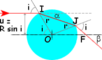
Crystal Balls (spherical lenses)
A solid sphere of glass (radius R, index n)
has focal length f = R/(2n-2)
There are several ways to obtain this result.
The easiest one is probably to notice that
the lens-maker's formula
(originally intended for thin
lenses only) applies directly to this particular case of a
thick lens, because of the existence of an
optical center
(a point through which light rays are not deflected at all).
We may also do it the hard way,
without even using the small-angle approximation:
For an incident ray at a distance u < R
from the center O of the sphere, we consider the plane xOy
where the x-axis is parallel to the ray
(whose direction is that of increasing values of x at a
constant value of y = u > 0).
See above figure.
The ray enters the sphere at point
I = ( x0 , y0 ) at an angle of incidence
denoted i
(that's the angle with respect to the normal to the surface).
x0 =
- ( R 2 - u 2 )½'
y0 = u = R sin i
The refracted ray emerges from I at an angle r
(with respect to the normal) whose sine is equal to u/nR
(according to Snell's law).
At this point, the ray's inclination with respect to the x-axis is
a (which is a negative angle).
sin r = (1/n) sin i = u / nR
a
= r - i
= Arcsin (u/nR)
-
Arcsin (u/R)
Using a dummy parameter z, the equations of the ray inside the sphere are:
x = x0 + z cos a
&
y = y0 + z sin a
The exit point J is at the nonzero value of z
for which x2 + y2 = R2 :
R 2 =
( x0 + z cos a )2 +
( y0 + z sin a )2
0 = z 2 +
2 z [
x0 cos a +
y0 sin a ]
Therefore, we must plug z = -2 [
x0 cos a +
y0 sin a ]
into the previous expressions
to obtain the coordinates
(x1 , y1 ) of the exit point J :
x1 = x0 - 2 [
x0 cos a +
y0 sin a ]
cos a
=
-
x0 cos 2a +
y0 sin 2a
y1 = y0 - 2 [
x0 cos a +
y0 sin a ]
sin a
=
-
x0 sin 2a +
y0 cos 2a
We could have obtained the same result geometrically...
Ransom
(2010-11-26)
Lens-Maker's Equation (with index n = 1.44)
Focal length of a lens with two concave faces of radii 0.300 & 0.970 m.
The following formula gives the focal length ( f )
for a thin lens made from stuff of index n
(relative to the surrounding medium)
bounded by two surfaces whose radii of curvature are respectively
R1 and R2
Lens-Maker's Formula
1
= (n-1) [
1
+
1
]
f
R1
R2
The curvatures are counted positively when the surface bends toward the
denser medium and negatively otherwise. Similarly, the resulting
focal length is positive for a converging lens and negative for a diverging one.
In the above case of a plastic
biconcave lens (n = 1.44) the radii
of curvature are both negative (-0.300 and -0.970). So is the
focal length given by the above formula:
f = -0.521 m
(2017-06-18) Thin-lenses are rectilinear.
With a rectilunear lens, the image of a straight line is a straight line.
For a thin-lens, the above shows fairly directly that the image of a plane
perpendicular to the optical axis is a plane perpendicular to the optical axis.
A straight line in such a plane is a line orthogonal to the optical axis
(it need not intersect it).
The image of a straight line orthogonal to the optical axis is another such line.
That's so because such a line can be defined as the intersection of a plane orthogonal to the axis
and a plane through the optical center (whose image is itself).
The image of the line is straight (and orthogonal to the optical axis)
as the intersection of the two corresponding image planes.
To complete our proof of rectilinearity, we'll now establish (the hard way)
that the image of the tilted line y = m x + b
in a plane containing the optical axis is indeed a straight line.
That will show that the image of a tilted plane is a tilted plane
(a tilted plane is formed by all orthogonal lines which intersect a given tilted line).
The final consequence will be that any striaght line has a straight image,
because it's at the intersection of two planes.
Here goes nothing: We choose our
coordinate system so that the x-axis is the optical axis and the plane of the lens is
at x = 0. Let (x',y') be the image of
a point (x.y) on the aforementioned line. We have:
y' / x' = y / x (An object point and its image are aligned with O.)
1 / x' - 1 / x = 1 / f (Thin-lens optical equation.)
To obtain a relation between x' and y' we'll
eliminate x and y from those three equations.
We start by eliminating y between the first two equations:
y' / x' = m + b / x
1 / x' - 1 / f = 1 / x
Now, we plug into the first equation the value of 1 /x given by the second:
y' / x' = m + b [ 1 / x' - 1 / f ]
Multiplying by x', we obtain: y' = ( m - b / f ) x' + b
This shows that the image of a straight line is a straight line which intersects it on the plane of the lens.
This result is the Scheimpflug principle:
An object on the plane y = mx + b has an image on y' = m'x' + b'
m' = m - b / f
b' = b
(2017-12-17) Galileo's refractor (Hans Lippershey, 1608)
The telescopic design which Galileo put to
astronomical use in 1609.
(2017-12-17) Reflecting telescope (Newton, 1668)
Overcoming the limitations of refracting telescopes.
Reflecting telescopes were proposed in the 17-th century to allow larger apertures
without the
chromatic aberration
inherent in the
dispersion of glass in lenses.
Also, a mirror only has one surface to polish instead of two.
Different designs were put forth:
All designs involve a large primary concave mirror and a smaller secondary mirror which
can be either convex, flat (Newtonian)
or concave (Gregorian).
The first reflecting telescope ever built was made by Newton
himself in 1668.
Newtonian telescopes feature a small flat mirror at a
45° angle to allow observation without significantly obstructing the primary mirror.
Newton's simple design is the optical basis for the so-called
Dobsonian telescopes
introduced around 1965 by amateur astronomer
John Dobson (1915-2014)
with simplified mechanical components which make
large-aperture telescopes more portable and/or more affordable:
Altazimuth mount (rocker box) and truss tube.
(2016-10-24) Microscopy (Antonie van Leeuwenhoek)
Optical Compound Microscope.
There are controversies about who actually invented the compound microscope
(two or more lenses mounted in a tube) but credit is often given to
Zacharias Janssen and/or
his father Hans Martens. Zacharias was born between 1580 and 1588
and he died sometime before his son Johannes got married (April 1632).
The earliest dates for the claim (1590 or 1595) looks dubious unless
the father was involved. There are no such reservations about the later part
of another reported range (1590 to 1618) which would still ensure priority.
What's for sure is that early compound microscopes were merely viewed as novelties
until Antonie van Leeuwenhoek put the invention to scientific use.
(2017-06-10) Imaging a tilted plane
(Jules Carpentier, 1901)
Scheimpflug and Hinge rules.
When the plane of the lens (orthogonal to the optical axis)
is tilted with respect to the film plane (film or
electronic sensor) the locus of all points
which are in sharp focus is a plane which intersects the
film plane on a straight line contained in the lens plane
(the Scheimpflug line ).
(2016-12-24) Light Falloff & Center Filters
Natural dimming away from the center of a photographic image.
This darkening of the sides of a photographic image is small for long lenses
or for retrofocal wide-angle lenses (as used in
small-format SLR cameras).
However, the effect is very noticeable with wide-angle lenses in large-format cameras.
It can be corrected with professional
center filters
costing hundreds of dollars.
Such filters (dark in the center and clear near the rim) must be manufactured with
precision to match a given lens.
In any camera with a thin-lens, the illumination of the image
falls off as the fourth power of the cosine
of the angular distance q to the optical axis
(as measured from the center of the lens)
for 3 combined reasons:
The intensity of light is inversely as the square of the distance to the source
(loosely speaking, the aperture of the lens acts as a source of light).
For a fairly narrow aperture, that distance is just inversely proportional to
cos q so the intensity is proportional to
cos2 q.
The amount of light received per unit area on the plate is proportional to the cosine
of its tilt from the rays. That's another factor of cos q.
Finally, the aperture is observed from the plate tilted at an angle of
q and its
apparent area is thus proportional
to cos q.
The maximum angle
q is half the field of view (corner to corner).
For a normal lens, the field of view is, by definition,
close to the field of view of the human eye, say
2q = 45°, which lets the above dimming factor be:
This means that the corners are about 0.457 f-stops dimmer than the center of
the image. Less than half a stop is noticeable but not striking
(for longer lenses, the effect is even harder to detect).
However, the situation is very different for wide-angle lenses, as shown by the following table:
Light falloff at corners, compared to the center of the image
(for a thin-lens)
(2016-12-24)
Retrofocus Wide-Angle Lens Design (Angénieux, 1950)
How to keep a lens with short focal length away from the focal plane.
The yet-to-be-named idea was first applied in the 1930's by
Taylor Hobson
for their Technicolor® cameras,
to provide space for the beam-splitter required by the Technicolor system.
This is also critical for single-lens-reflex (SLR) cameras,
to allow room for the flip-up mirror behind the lens.
(2015-06-01) Resolving Power
(Lagrange & Abbe)
Best possible resolution is inversely proportional to aperture.
This isn't part of proper geometrical optics but it's good
to know what limit to the sharpness of lenses is imposed by diffraction
(due to the wavelike nature of light).
The following formula gives the smallest angular distance between
two points that can be barely distinguished according to the conventional
Rayleigh's criterion.
For other conventions, a slightly different coefficient would be
substituted for the
Rayleigh factor (1.220).
(2008-10-26) Shadow Hiding. The Opposition Effect.
The cause of extra brightness directed back to the source of illumination.
When illuminated, a smooth enough dull surface sends back
in all directions an intensity of light which is proportional to
its apparent area in the direction of the observer
(Lambert's Law).
However, some features of a rough surface may be large enough to cast shadows
on deeper patches which reduce the percentage of the surface that's illuminated.
This can reduce significantly the albedo of the surface of a rocky planet
whenever it's not observed directly at opposition.
(2015-05-22) Honeycomb Grid Snoot Suppressing diverging rays from a beam.
The device consists of many circular tubes with imperfectly reflective walls,
parallel to the central axis of a light beam.
A ray entering such a tube isn't modified if it's almost parallel to the axis.
Otherwise, the ray is reflected n times off the walls of the tube and
emerges with the same angle (up to a change of sign when n is odd,
which we may ignore if we assume the system to be symmetric with respect to the
central axis, since two symmetric rays simply switch rôles in that case).
Because the material isn't perfectly reflective, each reflection reduces the
intensity of a ray by a factor k < 1.
The total attenuation is kn.

")
")


 (2015-05-22) Honeycomb Grid Snoot