(2012-02-15) Chebyshev Polynomials [ of the first kind ]
A family of commuting polynomial functions.
Tn oTp
= Tp oTn
= Tnp
cos(nq) is a polynomial
function of cos(q).
The following relation defines a polynomial of degree n
known as the Chebyshev polynomial of degree n:
cos (nq) =
Tn (cos q)
The symbol T comes from careful Russian transliterations like
Tchebyshev,
Tchebychef (French) or
Tschebyschow
(German).
Alternate spellings include
Tchebychev (French)
and "Chebychev".
The trigonometric formula
cos (n+2)q =
2 cos q cos (n+1)q -
cos nq
translates into a simple recurrence relation which makes Chebyshev polynomials
very easy to tabulate, namely:
T0 (x)
=
1
Tn+2 (x) =
2 x Tn+1 (x) - Tn (x)
T1 (x)
=
x
Pafnuty Chebyshev
T2 (x)
=
-1
+
2 x2
T3 (x)
=
-3 x
+
4 x3
T4 (x)
=
1
-
8 x2
+
8 x4
T5 (x)
=
5 x
-
20 x3
+
16 x5
T6 (x)
=
-1
+
18 x2
-
48 x4
+
32 x6
T7 (x)
=
-7 x
+
56 x3
-
112 x5
+
64 x7
T8 (x)
=
1
-
32 x2
+
160 x4
-
256 x6
+
128 x8
Knowing only the highest term of Tn and its obvious n distinct real zeroes,
we obtain immediately Tn as a product of n factors:
If n > 0, then Tn (x) = 2 n-1
n-1
( x - cos (k+½)
p/n )
Õ
k=0
The case Tn (0) = (-1)n tells
something nice about a product of cosines.
Inverse formulas :
x0
=
T0
x1
=
T1
2 x2
=
T0
+
T2
4 x3
=
3 T1
+
T3
8 x4
=
3 T0
+
4 T2
+
T4
16 x5
=
10 T1
+
5 T3
+
T5
32 x6
=
10 T0
+
15 T2
+
6 T4
+
T6
64 x7
=
35 T1
+
21 T3
+
7 T5
+
T7
128 x8
=
35 T0
+
56 T2
+
28 T4
+
8 T6
+
T8
(2014-07-26) A solution looking for a problem :
Chebyshev polynomials verify Tm(Tn(x)) =
Tmn(x). This unique property makes it possible to define pairs of
closely related functions from any pair of arithmetic functions u and v
(with subexponential growth) that are
Dirichlet inverses of each other,
using the following symmetrical relations:
¥
g ( x ) =
å
u(n) f ( Tn(x) )
n = 1
¥
f ( x ) =
å
v(n) g ( Tn(x) )
n = 1
If f (0) = 0,
those series are usually absolutely convergent,
because Tn(x) decreases exponentially with n,
for any fixed x in ]-1,+1[.
Proof :
Expand the latter right-hand-side using the definition of g :
å m
å n
u(n) v(m) f ( Tmn (x) )
=
å k
[
å d|k u(d) v(k/d)
]
f ( Tk (x) )
u and v being Dirichlet inverses,
the bracket is either 1 (if k = 1) or 0.
This applies, in particular, when u is a totally multiplicative
arithmetic function [i.e., such that u(mn) = u(m) u(n)
for any m & n ]
in which case its Dirichlet inverse can be expressed using the
Möbius function (m) :
v(n) = m(n) u(n)
Using Tn(x) = x1/n instead of Chebyshev polynomials,
this pattern was used in 1859 by Riemann to link
his (normalized) prime-counting function
f = p
with the celebrated jump function
g = J he obtained with u(n) = 1/n.
(2012-02-16) Laguerre Polynomials
Radial part of the solution of the Schrödinger equation
for hydrogenoids.
Laguerre's equation is a second-order linear differential equation:
x y'' + (1-x) y' + n y = 0
It has non-singular solutions only when n is a non-negative integer.
In that case, a solution is Ln(n), the Laguerre polynomial of order n
given by:
L0(x)
=
1
(n+1) Ln+l (x) = (2n+1-x) Ln (x) - n Ln-1 (x)
L1(x)
=
1
- x
2
L2(x)
=
2
- 4x
+ x2
6
L3(x)
=
6
- 18x
+ 9x2
- x3
24
L4(x)
=
24
- 96x
+ 72x2
- 16x3
+ x4
120
L5(x)
=
120
- 600x
+ 600x2
- 200x3
+ 25x4
- x5
720
L6(x)
=
720
- 4320x
+ 5400x2
- 2400x3
+ 450x4
- 36x5
+ x6
5040
L7(x)
=
5040
-35280x
+52920x2
-29400x3
+7350x4
-882x5
+49x6
-x7
Edmond Laguerre
Edmond Laguerre
(1834-1886; X1853) may have devised those polynomials
as early as 1860 but the relevant memoir was only published in 1879.
The Laguerre polynomials arose from a remarkable
continued fraction expansion
of the definite integral from zero to infinity of exp(x)/x
Generalization :
Sorin is credited for the following generalized Laguerre equation :
x y'' + (a+1-x) y' + n y = 0
This is satisfied by the Laguerre function, defined by:
L
(a) n
=
¥
(
n+a n-p
)
(-x)p p!
å
n=1
Because of the way binomial coefficients vanish,
a polynomial (a finite sum) called associated Laguerre polynomial
is so obtained when n is a non-negative integer.
Otherwise, the above is a divergent series which is
Borel-summable.
Ordinary Laguerre polynomials correspond to the special case
a = 0.
After deriving explicit formulas up to p = 17, Johann Faulhaber
observed that, if p = 2q+1 is odd,
then the sum of the p-th powers of the integers from 0 to n is
a polynomial of degree q+1 in the variable x = n(n+1)/2.
A related expression holds for a nonzero even p, namely:
n
å
k=0
k 2q+1
=
Fq+1(x)
If q > 0, then:
n
å
k=0
k 2q
=
n+½ 2q+1
d dx
Fq+1
(x)
That result was proved in full generality by
Carl Jacobi, in 1834.
(2020-06-02) Cyclotomic Polynomials
Irreducible divisors of x n - 1 over the rationals.
The nthcyclotomic polynomial
Fn is the unique monic polynomial dividing
x k - 1 for k = n
but not for any lesser value of k.
When n > 1, Fn is
palindromic.
If n has at most two distinct odd prime factors, then the
coefficients of Fn stay within {-1,0,1}.
That holds for n < 105; the first product of three distinct odd primes
(Adolph Migotti, 1883).
Those coefficients can be arbitrarily large
(Issai Schur, 1931).
Furthermore, any given integer occurs as a coefficient of some
cyclotomic polynomial (Jiro Suzuki,
1987).
Fn is an irreducible polynomial
over the rationals, whose degree is equal to the
Euler totient f (n).
That nontrivial fact is due to Carl F. Gauss.
The following definition also holds for n = 0
(as an empty product is 1).
Fn (x) =
Õ
(
x - exp( i 2kp / n)
)
1 ≤ k ≤ n GCD(k,n) = 1
For n > 0, the cyclotomic polynomial Fn
can thus be defined as the unique monic
polynomial whose roots are the primitive nth roots of unity.
Conditional proof in the 1934 thesis of Rolf Bungers,
possibly the future seismologist (1909-1942)
[former student of Gustav Angenheister (1878-1945)
who died in a plane crash in Norway, on 1942-12-24]
(2020-06-03) Lucas coefficients (Edouard Lucas, 1878)
Nontrivial factors of (p x2) p ± 1
when p is an odd prime.
A polynomial Pp can be defined for which the following identity holds,
which provides a nontrivial factorization of some special integers:
( p x2 ) p - (-1)m =
( p x2 - (-1)m ) Pp (-x) Pp (x)
Here, p = 2m+1 is an odd prime
(see Sophie Germain identity for p=2).
Pp (x) = Ap ( p x2 ) + (p x) Bp ( p x2 )
where Ap and Bp are both
palindromicmonic polynomials.
Ap has degree m. Bp has degree m-1.
Polynomials
Pp (x) = Ap (y) + (p x) Bp (y) with y = p x 2
±
Prime p
1
y
y2
y3
y4
y5
y6
y7
y8
y9
y10
y11
y12
y13
y14
y15
+
p=3
A
1
1
B
1
-
p=5
A
1
3
1
B
1
1
+
p=7
A
1
3
3
1
B
1
1
1
+
p=11
A
1
5
-1
-1
5
1
B
1
1
-1
1
1
-
p=13
A
1
7
15
19
15
7
1
B
1
3
5
5
3
1
-
p=17
A
1
9
11
-5
-15
-5
11
9
1
B
1
3
1
-3
-3
1
3
1
+
p=19
A
1
9
17
27
31
31
27
17
9
1
B
1
3
5
7
7
7
5
3
1
+
p=23
A
1
11
9
-19
-15
25
25
-15
-19
9
11
1
B
1
3
-1
-5
1
7
1
-5
-1
3
1
-
p=29
A
1
15
33
13
15
57
45
19
45
57
15
13
33
15
1
B
1
5
5
1
7
11
5
5
11
7
1
5
5
1
+
p=31
A
1
15
43
83
125
151
169
173
173
169
151
125
83
43
15
1
B
1
5
11
19
25
29
31
31
31
29
25
19
11
5
1
For p=31 (and x=9) this factors a nice 102-digit
semiprime: (251131+1) / 2512
= 889923919072997985238634558820908333948499157179463 × 1111413273683146858652465162019244587926917356315577
That factorization would take a long time with a
general-purpose program.
For compactness, we'll give palindromic polynomials as lists of coefficients
with underlined central ones (so the mirror endings can be freely truncated).
For p=61 (with x=2) this gives the
factorization
of the 144-digit semiprime (24461-1) / 35 =
254180335737792836487420059360430288526895310810588085366845580859576779
× 691880648894768106905652479597579967344338476040716833288367161850591919