Vocabulary :
For an objective function of several variables, a "stationary point"
is a set of values of those variables where all partial derivatives
of the function vanish.
As illustrated below, a local extremum must be
a stationary point but the converse need not hold.
Because of the inclusive meaning
assigned by default to the simplest mathematical terms
(which is the exact opposite of the exclusive meaning often
attributed to simple words in everyday language)
most mathematicians consider "stationary point" and "saddlepoint"
to be synonymous:
At a saddlepoint, the relevant quantity may
rise in some directions and fall in others
but it's not required to do so...
There might very well be an extremum there!
Some authors reserve the term "saddlepoint"
to nonextremal stationary points.
We prefer to call those proper
saddlepoints
(thus following normal mathematical nomenclature).
(2015-01-30) Optimizing before Calculus
Some historical cases have beautiful ad hoc solutions.
Without the general methods presented in the rest of this page,
every optimization problem appears to call for a brilliant insight.
Here are a few classical such solutions, which ought to be remembered not only for
the sheer beauty of the arguments leading to them but also for the
simplicity in which the final results can be described.
Arguably, ad hoc methods are best suited for problems whose
solutions are simple (like Dido's problem).
Once guessed, such solutions may have beautiful justifications.
In general, however, correctly guessing the solution of a complicated optimization problem
is all but impossible and calculus
is required for both the discovery and the justification
of the solutions. When calculus itself becomes difficult to apply,
the latest trend is to use numerical methods instead of symbolic manipulations
(this should only be a last resort, though).
The solution of our first optimization problem depends on what can be construed as
Euclid's postulated "optimization", namely:
Postulate :
In a Euclidean plane (or Euclidean space) the shortest path between two
points is a straight line.
Single-variable optimization: Laws of classical optics.
Heron's problem
(least length and laws of reflection):
In the plane, we consider a straight line and two points A and B
on the same side of the line.
The basic question is to find which point M
on the line will yield the shortest two-legged path from A to M
and M to B.
The key observation is that any such path has the same length as a path from A
to M and from M to the point B',
symmetric of B with respect to the line.
Conversely, any path from A to B' must cross the line at
a point M.
If the path from A to B' is shortest, so is the matching
path from A to M to B.
By postulate,
the shortest path from A to B' is a straight line and the
solution M is simply found as the intersection of two straight lines.
Heron thus showed, nearly 2000 years ago, that the main law of
mirror optics (the angle of reflection is equal to the angle
of incidence) can be deduced from the appealing postulate that light travels
along the shortest available route.
A great intellectual feat for that time, or for any time!
Fermat's principle
(least time and laws of refraction):
Postulating instead (more generally) that light travels along the fastest
route, the assumption that its speed is different on either side
of the line yields the basic law of refraction (Snell's law).
Two-variable optimization: Torricelli points.
The Torricelli point minimizes the sum of the distances
to three given points. (This is a two-dimensional specialization of Plateau's laws.)
(2007-09-23) Optimizing a smooth function f
of a single variable.
'Tis little more than finding where the function's
derivative vanishes.
For a point x in the interior
of the domain of f and a small enough value
of e,
both points x-e
and x+e are in the allowed domain and
yield values of f which are on both sides of
f (x) if we just assume that f'
is nonzero. Therefore, there can be an extremum at point x
only when f' (x) vanishes.
On the other hand, there's no such requirement for a point x
at the border of the allowed domain, because small displacements
of only one sign are allowed.
Away from the border, a saddlepoint x
(let's use that general term to indicate that
f' (x) vanishes) will be
the location of a
minimum (resp. a
maximum )
when f'' (x)
is positive (resp. negative).
If it's zero, further
analysis is needed to determine whether x
is the location of an extremum or not.
(It's indeed an extremum if the first nonzero derivative
is of even order.)
(2016-01-11) Angle maximization problem of Regiomontanus :
An historical example of a single-variable problem of the above type.
Regiomontanus (1436-1476)
proposed to discuss how a line segment is viewed at an angle
q from a variable viewpoint.
That angle is maximum (and equal to 180°) from a point inside the segment.
It is minimum (and equal to 0°) for a viewpoint on the same line as
the segment but outside of it.
The angle is arbitrarily small from viewpoints at large distances.
Regiomontanus considers a line perpendicular to the line of the segment and crossing it at
a point outside the segment. He asks when the viewing angle is maximum
from points on that line.
(E. M. of Wisconsin Rapids, WI. 2000-11-21)
Saddlepoints & Extrema
Determine the points where the [objective] function
z = 3x3+3y3-9xy
is maximized or minimized. [ Check for
second-order condition. ]
A necessary (but not sufficient) condition for a smooth function
of two variables to be extremal
( "minimized" or "maximized" ) on an open domain
is to be at a saddlepoint
where both partial derivatives vanish.
In this case that means:
9x2-9y = 0
and
9y2-9x = 0
So, extrema of z can only occur when
(x,y) is either (0,0) or (1,1).
To see whether a local extremum actually occurs,
we must examine the second-order behavior of the
function about each such saddlepoint
(in the rare case where the second-order
variation vanishes, further analysis would be required).
Well, if the second-order partial derivatives are L, M and N, then
the second-order variation at point (x+dx, y+dy) is the quantity
½ [ L(dx)2 + 2M(dxdy) + N (dy)2 ]
We recognize the bracket as a quadratic expression whose sign remains the same
(regardless of the ratio dy/dx) if and only if
its (reduced) discriminant(M2-LN) is negative.
If it's positive, the point in question is not an extremum.
In our example, we have L = 18x, M = -9 and N = 18y.
Therefore:
M2 - LN = 81 (1 - 4xy)
At (0,0) this quantity
is positive (+81).
Thus, there's no extremum there.
On the other hand, at the point (1,1)
this quantity is negative (-243) so the point (1,1) does
correspond to the only local extremum of z.
Is this a maximum or a minimum? Well, just look at the sign of L
(which is always the same as the sign of N for an extremum).
If it's positive, surrounding points yield higher values and,
therefore, you've got a minimum. If it's negative you've got a maximum.
Here, L = 18, so a minimum is achieved at (1,1).
To summarize: z has only one local extremum;
it's a minimum of -3, reached at x=1 and y=1.
Does this mean we have an absolute minimum?
Certainly not!
(When x and y are negative,
a large enough magnitude of either will make
z fall below any preset threshold.)
(2007-09-22) Unconstrained (or "absolute") saddlepoints
Saddlepoints of a function of several independent variables.
We're seeking saddlepoints (stationary points) of a
scalar objective function
M of n variables x1 , ... , xn
which we view as components of a vector x.
M ( x1 , ... , xn ) = M ( x )
If those n variables are independent,
then a saddlepoint is obtained only at a point where
the differential form dM vanishes.
This is to say:
0 = dM = grad M . dx
As this relation must hold for any
infinitesimal vectorial displacement
dx, such absolute saddlepoints of M
are thus characterized by:
grad M = 0
That vectorial relation is shorthand for
n separate scalar equations:
¶ M
= 0
¶xi
(2007-09-22) Lagrange Multipliers
Optimizing entails one Lagrange multiplier per constraint.
Instead of a set of independent variables
(as discussed above) we may have to deal with several
variables tied to each other by several constraints.
The method of choice was originally introduced by
Lagrange (before 1788)
as an elegant way to deal with mechanical constraints:
For example, the variables may be subject to a single constraint
(e.g., the cartesian equation of a surface on which a point-mass is free to move).
E ( x1 , ... , xn ) = constant
While an unconstrained saddlepoint
of M was obtained when dM = 0.
A constrained saddlepoint is obtained when dM is proportional to dE.
More generally, when k functions
E1 ... Ek are given to be constant,
a constrained saddlepoint of M is achieved when the
differential form dM is a linear
combination of the differentials of E1 ... Ek.
dM =
l1 dE1 +
l2 dE1 + ... +
lk dEk
In other words, there are k constants
li
(each is known as the Lagrange multiplier
associated with the corresponding constraint) such that the following
function has an unconstrained (or absolute)
saddlepoint.
(2007-09-23) The fattest cone of given base...
What apex minimizes the lateral area of a cone of given base and volume?
The volume of a cone is one third of the product of its base area by its
height. So, by imposing the cone's volume, we're actually imposing
the height of the cone and looking for an optimal
apex somewhere in a fixed plane parallel to the base...
(2007-09-23) Calculus of Variations
(cf. Lagrangian mechanics)
Euler-Lagrange equations hold whenever a path integral is stationary.
Historically,
the first problem of the type described below
was the brachistochrone problem
(find the shape of the curve of fastest descent)
which had been considered by Galileo
in 1638 and solved by Johann Bernoulli in 1696
(Bernoulli withheld his solution to turn the problem into a public challenge,
which was quickly met by several prestigious mathematicians).
The subject was investigated by Euler in 1744 and
by Lagrange in 1760.
It was named calculus of variations by Euler in 1766
and made fully rigorous by Weierstrass
before 1890.
Let L be a smooth enough function
of 2n+1 variables:
L =
L ( q 1 , q 2 ... q n ,
v1 , v2 ... vn , t )
We assume that the first n variables (q) are actually functions of the
last one (t) and also that the subsequent variables (v)
are simply their respective derivatives with respect to t:
v i (t) =
d
q i (t)
dt
This makes L a function of t alone and we may consider
the following integral S (called the "action" of L )
for prescribed configurations at both extremities.
In this context, a configuration is defined as a complete set
of values for the q-variables only (irrespective of what the v-variables may be)
so, what we are really considering now are prescribed fixed values of
all the 2n quantities
q i (a) and
q i (b).
S =
ò
b
L dt
a
The fundamental problem of the calculus of variations is to
find what local conditions make S stationary,
for optimal functions q i .
Namely:
Euler-Lagrange equations
¶L
=
d
(
¶L
)
¶ q i
dt
¶ vi
Proof :
From a set of optimal functions q i
and arbitrary (sufficiently smooth) functions
h i which vanish at both extremities
a and b, let's define the following family of
functions, depending on one parameter e :
Q i (t) = q i (t) +
e h i (t)
V i (t) = v i (t) +
e
d
h i (t)
dt
Those yield a value S(e) of the action which must be
stationary at e = 0
(since the functions q i
are optimal). Thus, the derivative of S(e)
along e does vanish
at e = 0, which is to say:
0 =
ò
b
å i
[
h i
¶L
+
d h i
¶L
] dt
a
¶ q i
dt
¶ vi
Since every h i vanishes at both extremities
a and b , we may
integrate by parts
the second term of the square bracket to obtain:
0 =
ò
b
å i
h i
[
¶L
-
d
(
¶L
)
] dt
a
¶ q i
dt
¶ vi
As h i is arbitrary, the square bracket must vanish
everywhere, for every i.
(If this wasn't so, the whole equality would be violated for a choice
of h i vanishing wherever the square bracket
doesn't have a prescribed sign).
Theoretical and Practical Examples :
The above is most commonly used as the basis for
variational mechanics and
related aspects of theoretical physics based on a
principle of least action.
However, it's also the correct answer to more practical concerns:
On 2008-10-27,
Bill Swearer
wrote: [edited summary]
As a pilot, I've always been interested in writing a proper piece of
flight-planning software to optimize the plane's path with regard to time, fuel,
or any combination thereof. [...]
I've always felt the professionally-provided solutions were crude approximations that do
not take into account the full range of possibilities, especially over long distance,
as one crosses varying jet streams at different altitudes, etc. [...]
What is the correct mathematical approach?
Thanks a lot. Bill Swearer
Well, just express carefully the local cost function
(L) as a function of the position of the aicraft and of the related derivatives
(to a good approximation, the latter are only useful to compute horizontal speed).
Predicted meteorological conditions (changing with time
throughout space) can be used for best planning.
The Euler-Lagrange equations then tell the pilot what to do at all times.
(2009-07-05) A Proof of Noether's Theorem (1915)
Proving Noether's theorem for continuous symmetries.
A slight modification of the above proof yields a straight
derivation of one of the
greatest statements of mathematical physics. Let's just do it...
Suppose that, for specific functions
hi , a symmetry exists which leaves L
unchanged, (to first-order in e about 0)
when q i is replaced by
Q i = q i +
e h i
Formally, this leads to a situation similar to the previous one,
since we still know that the derivative of
S(e) vanishes at
e = 0
(albeit for very different reasons).
However, the h functions need not vanish at the extremities
a and b.
So, an extra "integrated term" appears
in the following expression of the derivative of
S(e)
which results from our integration by parts:
0 =
å i
h i
¶L
|
b
+
ò
b
å i
h i
[
¶L
-
d
(
¶L
)
] dt
¶ vi
a
a
¶ q i
dt
¶ vi
Now, as the integral still vanishes (because
the previously established Euler-Lagrange equations make every
square bracket vanish) the extra term must be zero as well.
This means that the following quantity doesn't change:
(2012-04-02) The geodesics of a two-dimensional surface.
Paths of least length.
On a 2D surface M (u,v) the infinitesimal
distance corresponding to a displacement du,dv is given by
the first fundamental quadratic form:
F1 (du,dv)
= (dM)2
= E (du)2 + 2 F du dv + G (dv)2
The problem of minimizing the length of the path between two points on that surface is
a standard exemple of the calculus of variations.
Let's introduce notations compatible with the above:
q1 = u
q2 = v
v1 = du/dt
v2 = dv/dt
L = [ F1 (v1 , v2 )
]½
=
[ E v12 + 2 F v1 v2
+ G v22
]½
(2010-07-06) The brachistochrone curve is a cycloid (1696)
The curve of fastest descent in a uniform gravitational field.
We are now presenting the brachistochrone problem as a simple application
of the calculus of variation. Historically, the relation is reversed,
as this problem actually helped define the need for the latter, which was formalized
many years after the brachistochrone problem was solved.
In June 1696,
Johann Bernoulli (1667-1748) challenged
the readers of Acta Eruditorum
with his famous brachistochrone problem:
Along what curve would a point-mass fall from one prescribed point to another lower
one (not directly underneath) in the least possible time?
Johann Bernoulli's own solution was published in the same journal
a year later, along with 4 of the 5 solutions sent by famous contributors
(the solution of Guillaume
de l'Hôpital was only published in 1988).
We shall use a coordinate system where the origin is the starting point.
We choose to orient the y-axis downward so that y is positive for
all target points. Let's call u the slope of the trajectory dy/dx.
In a gravitational field g the conservation of mechanical energy for a mass
m dropped from the origin at zero speed tells us that:
m g y = ½ m [ (dx/dt)2 + (dy/dt)2 ]
Therefore, ( 2 g y ) ½ dt = ( 1 + u2 ) ½ dx
To minimize the descent time, we seek to minimize the path integral of dt or, equivalently,
to minimize the integral of (2g)½ dt = L dx
(2016-01-11) Dido's Problem
Idealized legendary real-estate deal upon which Carthage was founded.
They purchased a site, which was named 'Bull's Hide' after the bargain
by which they should get as much land as they could enclose with a bull's hide.
Aeneid by
Virgil (70-19 BC)
The land so acquired by
queen Dido,
founder Carthage,
is interpreted to be whatever area could be bounded by the seashore on one side and a
rope of fixed length on the other.
(The preliminary step was to cut the hide into very thin strips to make a long rope out of it.)
The problem is to maximize that area, assuming the shore line to be perfectly straight.
To prove that the solution is a half-circle, one considers the two straight lines drawn
from an arbitrary point on the optimal boundary to either extremity of the rope
(on the shoreline). If we assume that both parts of the rope are rigidly attached
to those two lines, there's a constant area between those lines and their respective ropes.
What remains is the area of the triangle formed
by two sides of fixed length and part of the shore line.
This area is greatest when the two sides are perpendicular!
By the second theorem of Thales,
a planar curve where an arbitrary point always sees the extremities at
a right-angle is a semicircle.
The isometric inequality is a corollary of Dido's solution :
In 1846, the great Swiss geometer Jakob Steiner
(1796-1863) showed that the above solution of Dido's problem implies the familiar
2-dimensional isoperimetric inequality
(i.e., the planar curve of given perimeter
which encloses the greatest area is a circle). Three steps:
The optimal shape is convex (or else its convex hull
would have lesser perimeter and greater area).
If two points cut the perimeter of an optimal convex shape in half,
the straight line joining them necessarily cuts the shape into two portions of equal area.
(Otherwise a better shape could be formed using two parts congruent to the
larger portion.)
As solutions of Dido's problem, both halves
must be semicircles. Therefore, the whole shape is a circle.
No such simple geometric solutions are available to justify the higher-dimensional
counterparts of the isoperimetric inequality, discussed next.
(2008-11-10) The Isoperimetric Inequality and its Generalizations
Among planar loops of unit length, the circle encloses the largest area.
The surface area S enclosed by a closed planar curve
of given perimeter P is largest in the case of a circle.
This ancient statement (proved geometrically by Steiner, in 1846)
can be expressed by the following relation, known as the isoperimetric inequality:
S ≤ P 2/ 4p
Generalizations to Higher Dimensions :
The three-dimensional equivalent of the isoperimetric inequality says that the
closed surface of area S which encloses the largest volume
V is a sphere.
V 2 ≤ S 3/ 36 p
The above can be generalized to n dimensions:
No hypersurface of hyperarea S encloses a larger
hypervolume V than the hypersphere.
This makes the relations given in the
oldest Numericana article yield:
(2008-11-10) Plateau's Problem. Minimal surfaces with given borders.
The mean curvature of a soap film is constant.
That constant vanishes when both sides of the soap film are at the same pressure,
in which case the film is a surface of least area within the given border.
However, the non-vanishing case was also considered by Joseph Plateau;
it arises when soap film encloses pockets of air...
Besides the familiar spherical soap bubble, the simplest case is a soap bubble
merged within a large planar film. It takes on the form of two spherical
caps which form an outer angle of 120°
(inner angle of 60°) with the planar part of the film
whwere they meet.
The thickness 2h and the equatorial diameter d of the
lenticular bubble are proportional to the radius of curvature of the spherical parts:
d
=
R
2h
=
(2-Ö3) R
= 0.267949...R
The Plateau rules (1873)
state that the solutions are smooth surfaces of
constant mean curvature with
only two possible types of inner singularities:
Lines where 3 such surfaces meet at equal angles (120°).
Isolated points
where 4 such lines meet at equal angles q.
Because a regular tetrahedron is formed by every other vertex of a cube,
two vertices of a regular tetrahedron
are seen from its center at the same angular separation as between
(1,1,1) and (1,-1,-1). The cosine of that angle is -1/3.
Chemists call it the tetrahedral angle :
Jean Taylor (1944-) published a proof of Plateau's laws in 1976.
Euler's catenoid (1741) :
By finding that the
catenoid is the only minimal
surface of revolution (besides planes orthogonal to the axis)
Euler solved Plateau's problem
(well before it was so named) when the given border consists of
a pair of two sufficiently close coaxial circles.
When the parallel planes of the coaxial circles are too far apart,
no catenoid can join them and the solution of Plateau's problem
just consists of separate planar surfaces.
A surface, found by
Riemann in 1860, consisting of
infinitely many horizontal planes with slanted tunnels between adjacent pairs.
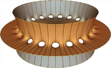
In 1982,
Celso
J. Costa
(a graduate student from Brazil) stumbled upon a
minimal surface topologically equivalent to a 3-hole torus.
Costa suspected that his surface had no self-intersections but,
at first, couldn't prove it...
David Hoffman teamed up with
William
H. Meeks III .
and
Jim Hoffman,
(then a graduate student) to produce a computer visualization of the
stunning symmetries of the strange surface described by Costa
(which contains two straight lines meeting at a right angle).
Dividing Costa's surface into 8 congruent pieces,
they proved, indeed, that it never intersects itself!
Loosely speaking, Costa's surface features two complementary
pairs of "tunnels" through the
equatorial plane which connect the inside of some "catenoidal" northern half
and the outside of its southern half, or vice-versa.
Subsequently, Dave Hoffman and Bill Meeks discovered that Costa's surface is just the simplest
member of a whole family of complete minimal
embedded surfaces constructed in the same way but with more "tunnels"...
Applied to helicoids, the idea yields yet another family of complete minimal
embedded surfaces where tunnels provide shortcuts between
slices of space which are otherwise connected only by circling around the helicoid's axis.
Denis Viala (2008-02-28) Connect the dots, without crossings...
Given n blue dots and n red dots in the plane (no three aligned)
there are always n disjoint segments with blue and red extremities.
Proof.
(HINT: This puzzle appears among optimization problems.)
(2008-11-09) Torricelli Points
Connecting three dots with lines of least total length.
The three vertices of a triangle ABC
can be connected using just its two shortest sides.
If the angle between those two sides is 120°
or larger, this is the most economical way to do so.
Otherwise, we may define a fourth point T such that
the three angles ATB, BTC and CTA
are all equal to 120°.
Then, the three llines TA, TB and TC form the most economical
way to connect the three dots A, B and C.
The point T is called
the Torricelli point of ABC.
The results for the first and the second of the above cases are unified
by defining T to be the vertex opposite the longest side
in the first case.
Likewise, four points in a plane are best connected by introducing
0, 1 or 2 new Torricelli points.
(2008-11-09) The Honeycomb Theorem
In 1999, Thomas Hales finally proved an "obvious" fact.
Nobody questioned
the celebrated Honeycomb conjecture
before 1993, when Phelan and Weaire showed its
3D counterpart (Kelvin's conjecture)
to be false!
The issue was settled in
1999
with a proper proof by Thomas C. Hales :
Thus, the 2D Honeycomb conjecture
is now a theorem! Here it is:
Honeycomb Theorem
In any partition of the plane into tiles of unit area,
each tile cannot have a lesser perimeter than the regular hexagon
of unit area.
(Loosely speaking, the regular honeycomb tiling
is the most economical one.)
The first proof by
Thomas C. Hales
(1999)
was surprisingly intricate.
It was crucial to get rid of the
convexity restriction which earlier authors had reluctantly imposed.
(The isoperimetric inequality
implies that the boundaries between
optimal shapes are either circular arcs or straight lines.
Both sides of such a boundary are convex only in the latter case.)
The reason curved boundaries are ruled out
is not at all obvious; it is false
in the 3D case.
(2015-01-10) Highly-symmetric monkey saddles of minimal area.
Surfaces whose borders have mirror-symmetry and an odd ternary axis.
With a vertical axis, such a curve has a vertical plane of symmetry,
the vertical coordinate is unchanged by rotation of
2p/3 (1/3 of a turn)
and its sign changes for half of that
(p/3 rotation).
A surface containing that line and having the same symmetry will be described by
an equation of the following type, in cylindrical coordinates:
z = f ( r , sin 3q )
[ f being odd for either argument ]
Let's find the functions f which make the
mean curvature constant:
(2008-11-09) Foam cells of unit volume and minimal area.
Kelvin's problem & counterexamples to Kelvin's conjecture.
Kelvin's problem is to partition space into unit-volume cells with least
surface area.
Simon Lhuilier
(1750-1840) called this one of the most difficult problems in geometry.
The uniform truncated octahedron
can tile space without voids.
Lord Kelvin (1824-1907)
observed that a partition of space into
Archimedeantruncated octahedra
was quite economical. He used the vertices as the basis for a proper foam,
with curved faces and edges engineered to
satisfy Plateau's rules.
The tetragonal faces of Kelvin's cell are planar figures whose
curved edges meet at the magic angle of 109.47122°.
The hexagonal walls are monkey saddles
with straight diagonals.
In 1887, Kelvin conjectured that his foam was the answer to the above optimization problem.
In the straight polyhedron, the angle q
between a square and an adjoining hexagon is slightly less than 60°.
An easy way to obtain the exact value is to consider the cube formed by the six
square faces. Seen from the center, the middles of the hexagons are in the directions
of the corners of that cube. Therefore:
q =
acos ( 1/Ö3 ) = 54.73561...°
By Plateau's rules, an optimally curved hexagonal surface always
meets the plane of an adjoining tetragonal face at an angle of 60°.
Therefore, the curved surface at the middle of an edge is inclined
5.26439° with respect to the plane of the original flat hexagon.
On the other hand, an edge between two hexagonal faces curves inward.
(It's the outward-curving edge of a tetragon in an adjacent cell.)
Although the equal-volume foams discussed below are more economical than this one,
Kelvin's foam remains best among all monohedral foams
(i.e., foams whose cells are all congruent to each other).
On the division of space with minimum partitional area
Sir William Thomson (Lord Kelvin).
Acta Mathematica, 11 (1887) pp. 121-134.
When a foam isn't monohedral, it need not be
equal-pressure. Actually, none of the foams below are.
In all of them, different cells may be assigned different "pressures" so a face's
mean curvature is the difference between
the pressures of the cells it separates (not necessarily zero).
In 1993, Denis Weaire (1942-)
and his student Robert Phelan disproved Kelvin's conjecture with a structure
more economical than Kelvin's foam:
The A15 Weaire-Phelan
structure is one example of a Frank-Kasper foam.
It consists of two distinct types of cells, with
pentagonal or hexagonal faces.
One cell is a squashed dodecahedron, the other is a tetradecahedron.
That basic structure occurs naturally in crystals of b tungsten.
In a draft
(2008-10-25)
of a paper published on
2009-06-02,
Ruggero Gabbrielli presents
a new type of unit-cell foam (featuring some tetragonal
faces) whose cost (5.303) is intermediate between
the Weaire-Phelan foam (5.288) and Kelvin's foam (5.306).
He calls this structure "P42a".
The repeating pattern consists of 14 curved
cells of 4 different types
(ten tetradecahedra and four tridecahedra).
It has an average
of 96/7 = 13.714285... faces per cell.
The above pictures for the A15 and P42a foams were
obtained by Ruggero Gabbrielli using the
GAVROG 3dt visualization software.
Gabbrielli has also posted several related
interactive
3D visualizations
under Java.
The 1993 optimization on A15 and Gabbrielli's recent research both used Ken Brakke's
Surface Evolver
(with specific code provided by John M. Sullivan, in the latter case at least).
At this writing, the A15 foam described by Weaire and Phelan in
1993 is still conjectured to be the answer to Kelvin's problem.
It is about 0.3% less costly than Kelvin's original foam.
The Weaire-Phelan foam was used as the basis for the design of the celebrated
Water-cube
of the 2008 Olympics
(Beijing National Aquatics Center) which is the largest structure
covered with ETFE film.
(2018-06-17) The Thomson Problem
What spherical distributions of N charges minimize potential energy?
J.J. Thomson is credited with the
discovery of the electron in 1897 (to be fair,
Jean Perrin had discovered it two years earlier).
This was the first subatomic particle ever discovered.
For quite a while, nobody knew exactly how neutral atoms could be made from those negative
electrons and some unknown positive stuff.
Thomson himself envisioned a naive model which became known as the
Plum-pudding model (1904)
whereby mutually-repulsive electrons would sit at the surface of a spherical blob of positive stuff.
In 1909, the celebrated gold-foil experiment was
conducted by Geiger and Marsden under the supervision of Ernest
Rutherford (1871-1937).
The observed violent bouncing of some of the alpha-particle projectiles suggested a totally different
model (Rutherford, 1911) where most of the atom's mass
resides in a tiny positively-charged nucleus around which electrons are maintained
in orbit by electric attraction.
Classically,
such accelerated charges would radiate energy away and the orbiting electrons would quickly spiral into
the nucleus... It was a major achievement of early
quantum mechanics to explain why they don't do so
(Bohr, 1913).
Back in 1904, J.J. Thomson wondered how N like charges would be distributed
on the surface of a sphere at equilibrium (minimizing potential energy,
at least locally). He set it as a purely mathematical puzzle, mostly for the
Coulomb potential (1/r) but possibly for other potentials as well.
Until 2010, the only known analytical solutions were the obvious configurations
for 1, 2, 3, 4, 6 and 12 charges (forming a
Platonic solid in the last three cases).
It was proved only recently (2010) that the triangular dipyramid
is the only solution for 5 charges.
Surprisingly enough, the Platonic solids for N = 8 or 20 are
not solutions (better distributions have been found numerically).
For example, for N=8, the cube is improved upon by a
square antiprism obtained from that cube by rotating
two opposing faces 45° from each other (about their common axis).
That shape happens to be optimal for the Coulomb potential.