Related Links (Outside this Site)

(2005-08-20)   Rationalized Beaufort Wind Scale
In "force n" weather, the wind speed is proportional to   n^3/2  =  nÖn

The widely-used  Beaufort scale  was devised in 1806, by Sir Francis Beaufort (1774-1857), rear admiral, hydrographer to the Royal Navy.  It was adopted by the British Admiralty in 1838, and has been in international use since 1874.  Originally, the Beaufort Wind Scale did not refer to specific wind speeds, but to the effect of the wind on a full-rigged ship, and the amount of sail which should be carried.  Since "force 12" meant a wind that 'no canvas can withstand', the original scale did not extend beyond that point.

Each Beaufort number still corresponds to a variety of common observations which can be made at sea or inland.  For example, in a "force 0" condition:  'Smoke rises vertically. Sea is like a mirror.'

Since 1946, the Beaufort scale has been defined in terms of the speed of the wind, measured by an anemometer placed 10 meters above the ground.

"Force n" means a wind speed around  V.n^3/2,  where V is a speed of about 1.871 mph  (we're told that the 1946 scale was officially based on a speed of 0.836 m/s, or about 1.87008 mph, which is slightly too low to be consistent with modern tables).  Any speed  V, in mph, between 62Ö26/169 and 146Ö46/529 yields agreement with the rounded "mph" scale below  (and also with the "km/h" scale, which is somewhat less restrictive).

Most tables  erroneously  give 18 mph instead of 17 mph as the upper limit for a moderate breeze; this is inconsistent with the rest of the table, for any value of  V.

To find the Beaufort number corresponding to a given speed, one divides that speed by V, and finds the whole number closest to the cubic root of the square of that ratio.  As a result of this modern definition, the Beaufort scale can be extended beyond the traditional limit of "force 12" for extremely violent winds.

We have not traced the existence of a "standard" value of V; we shall simply note that a value V = 0.8365 m/s (or any value between 0.83626 m/s and 0.8368 m/s) will agree with the above tables in mph or km/h, but that (inexplicably) tables published in knots imply a value of V falling in the incompatible range of 0.8401 m/s to 0.8433 m/s (once the inconsistent value of 16 knots published for the upper limit of a moderate breeze is lowered to 15 knots).

Wheather reports for sailors commonly use the Beaufort scale or quote wind speeds in knots.  Otherwise, the media may prefer different units for wind speeds in different parts of the World:  m/s (Sweden, Denmark), km/h (France, Germany, Canada), mph (United States).

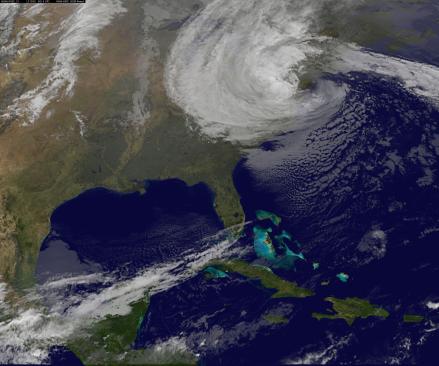
(2005-08-20)   Saffir-Simpson Hurricane Scale   (SSHS)
The customary scales for hurricanes  (Beaufort  force 12  and "above").

In August 1969, Hurricane "Camille" hit the Mississipi-Alabama coast with what would be "force 23" winds in an extended Beaufort scale:  200 mph to 213 mph.  However, the Beaufort scale is rarely extended  (if ever)  beyond force 12.  Instead, the strength of hurricanes is described with the following scale, which was originally devised in 1969 by Herbert Saffir (1917-2007)  a consulting structural engineer,  and   Dr. Robert H. Simpson (b. 1912) director of the  National Hurricane Center  (NHC)  from 1967 to 1974.

The  NHC  considers anything below category 1 to be either a  tropical depression  (D)  or a  tropical storm  (S).  Categories 1 and 2 are  Hurricanes  (H)  above the Beaufort  force 12  threshold.  Categories 3, 4 and 5 are  major hurricanes  (M).  There's no need for a category 6.

The above pressures and surge heights  (estimated by Bob Simpson)  were originally part of the  SSHS  definition.  However, in 2009, the NHC moved to base the definition of the  SSHS  purely on wind speeds  (expressed in knots,  kt).  The new scale is unambiguously called  Saffir-Simpson Hurricane Wind Scale  (SSHWS).  It became effective on 2010-05-15 and was revised on 2012-05-15.

In the Atlantic, the record-breaking hurricane season of 2005 included three category-5 hurricanes, named Katrina, Rita and Wilma (in chronological order).  At this writing (Oct. 2005) Wilma is the most intense hurricane ever observed in the Atlantic basin, featuring the lowest sea-level atmospheric pressure ever recorded in the Western Hemisphere outside of tornadoes  (882 hPa).  In the Northwest Pacific Ocean, only 9  typhoons  have surpassed the intensity of Wilma.  (The terms  typhoon  and  hurricane  describe the same phenomenon, but are used in different parts of the Globe.)

The costliest hurricane ever was  hurricane Katrina  (August 23 to 31, 2005) which caused an estimated $200 billion in damages and at least 1281 fatalities  (official count at this writing).  After hitting land as a mere category-1 hurricane north of Miami on August 25, the eye of Katrina made landfall again in Louisiana at 6:10am (CDT) on Monday, August 29, 2005.  as a category-4 hurricane...  By 11 am, the storm surge had breached the levee system protecting  New Orleans  from Lake Pontchartrain.  Most of the city was subsequently flooded.

Hurricane Names

The names of Hurricanes comes from a preapproved yearly list of 21 names with initials A through W (skipping Q and U) which is reused every 6 years, except that names of violent hurricanes are retired and replaced...  The 2005 season had so many major storms that the last ones had to be named after letters from the Greek alphabet  (Alpha, Beta, Gamma, Delta, Epsilon, Zeta).

The list of retired names is typically decided in March of the following year.  At this writing (2012-10-28, 11am EDT) there are great fears that  Hurricane Sandy  will make the list, as it threatens New-York City and other areas to the North of the region commonly affected by Atlantic hurricanes.  It made landfall in New-Jersey on Monday night (2012-10-29) after falling just below hurricane strength.

The following names have been retired, before the 2019 season:   Agnes (1972), Alicia (1983), Allen (1980), Allison (2001), Andrew (1992), Anita (1977), Audrey (1957), Betsy (1965), Beulah (1967), Bob (1991), Camille (1969), Carla (1961), Carmen (1974), Carol (1954), Celia (1970), Cesar (1996), Charley (2004), Cleo (1964), Connie (1955), David (1979), Dean (2007), Dennis (2005), Diana (1990), Diane (1955), Donna (1960), Dora (1964), Dorian (2019), Edna (1968), Elena (1985), Eloise (1975), Erika (2015), Fabian (2003), Felix (2007), Fifi (1974), Flora (1963), Floyd (1999), Fran (1996), Frances (2004), Frederic (1979), Georges (1998), Gilbert (1988), Gloria (1985), Gracie (1959), Gustav (2008), Harvey (2017), Hattie (1961), Hazel (1954), Hilda (1964), Hortense (1996), Hugo (1989), Igor (2010), Ike (2008), Inez (1966), Ingrid (2013), Ione (1955), Irene (2011), Iris (2001), Irma (2017), Isabel (2003), Isidore (2002), Ivan (2004), Janet (1955), Jeanne (2004), Joan (1988), Joaquin (2015), Juan (2003), Katrina (2005), Keith (2000), Klaus (1990), Lenny (1999), Lili (2002), Luis (1995), Maria (2017), Marilyn (1995), Matthew (2016), Michelle (2001), Mitch (1998), Nate (2017), Noel (2007), Opal (1995), Otto (2016), Paloma (2008), Rita (2005), Roxanne (1995), Sandy (2012), Stan (2005), Tomas (2010) and Wilma (2005).

Because of the COVID-19 pandemic, the week-long WMO Committe couldn't be held normally in the Spring of 2020 to officially retire Dorian.  Other possible retirees from the 2019 season include Imelda and Lorenzo.

Saffir-Simpson Hurricane Scale (SSHS & SSHWS)   |   List of tropical cyclone names
 
L'Ouragan Irma, c'est quoi? (6:15, French)  by  Dr Nozman  (2017-09-22).

(2005-08-20)   Fujita scale for tornadoes
Local twisters are primarily measured against a 6-rung scale  (F0 to F5).

Within tornadoes, the wind can reach speeds in excess of 280 mph  (450 km/h).  If the Beaufort scale was applicable, this would mean force 28 or 29.  Instead, all tornadoes are ranked using the following scale, from weakest to strongest, which was devised in 1971 by Ted Fujita (1920-1998) at the University of Chicago.

The Original Fujita Tornado Scale  (1971-2007)

Fn	Effects	Wind speed  (km/h)
F0	Twisted antennas, broken branches	60 to 110
F1	Uprooted trees, vehicles turned over	120 to 170
F2	Lifted roofs, small projectiles	180 to 250
F3	Walls tipped over, large projectiles	260 to 330
F4	Houses destroyed, some trees lifted	340 to 410
F5	Large structures lifted, incredible damages	420 to 510

Since February 1, 2007, a revised scale has been used which is known as the  Enhanced Fujita  scale (EF).

The Enhanced Fujita Tornado Scale

EFn	Effects	Wind
EF0	Minor damage.  Some roof damage, shallow trees knocked over, etc.	65 to 85 mph
EF1	Moderate damage.  Roofs stripped, mobile homes turned over, windows broken.	86 to 110 mph
EF2	Considerable damage.  Cars lifted off the ground, roofs torn off houses, large trees uprooted.	111 to 135 mph
EF3	Reports of well-constructed houses totaled, trains and big rigs overturned, heavy cars thrown off ground.	136 to 165 mph
EF4	Houses and whole frame houses completely leveled, cars thrown and small missiles generated.	166 to 200 mph
EF5	Houses and frames swept away, steel enforced concrete structures badly damaged.  Cars thrown like toys.	over 200 mph

What are the various degrees of tornadoes? (Yahoo!  Answers)

(2006-12-02)   Measuring in Decibels  (dB)
A general-purpose logarithmic scale for physical  power.

In a given medium, a signal carries a certain power  (or a power flux)  proportional to the square of an associated "amplitude"  (which may be variously defined).

The "amplitude" of an oscillating linear system is preferably defined as the  RMS of an  intensive  quantity  (like voltage).  The square of that amplitude divided by the RMS of the corresponding power is called "impedance".  If we divide by a power flux instead, what we obtain is known as a "characteristic impedance" (see below the example of sound, where the amplitude is a pressure).  Conversely, since the characteristic impedance of the vacuum is traditionally expressed in ohms  (it's 376.73...W)  the "amplitude" of the electromagnetic field should be expressed in V/m, which identifies the electric field (E).

The  relative magnitude  of two signals may be expressed equivalently as a logarithmic function of the ratios of their powers (P) or as the same logarithmic function of the squares of their amplitudes (A).  If decibels (dB) are used, the  relative  magnitude of the signal  (compared to some other signal of reference)  is defined by either of the following expressions, which involve  decimal  logarithms.

Relative magnitude (or  level)  in dB   =   10  log( P/P₀ )   =   20  log( A/A₀ )

When the amplitude  doubles,  the power becomes  4 times  as high and the level is raised by  roughly  6 dB.  If the amplitude is multiplied by 10, the power is 100 times higher and the level is raised exactly 20 dB.

From relative ratios to absolute measurements :

Decibels are most useful to express ratios of related signals  (for example the signals at the input and the output of an electronic amplifier).  However, specifying a conventional "reference" signal readily establishes an "absolute" decibel scale.  Each choice of a particular reference establishes a different "absolute" scale. 

The most popular such scale  (especially among electrical engineers)  is the  decibel-milliwatt  (dBm)  for which the zero level (0 dBm) is a signal whose total (harmonic) power is one milliwatt  (1 mW).

L   =   10  log ( P / 1 mW )  dBm

Power (P)	0.1 mW	1 mW	10 mW	100 mW	1 W	10 W
Level (L)	-10 dBm	0 dBm	10 dBm	20 dBm	30 dBm	40 dBm
	-40 dBW	-30 dBW	-20 dBW	-10 dBW	0 dBW	10 dBW

(2010-01-03)   Measuring Sound in Decibels  (dB)
Sound Intensity Level  (SIL)  and  Sound Pressure Level  (SPL)

As sound propagates, it carries a certain power per unit area of a small surface perpendicular to the direction of propagation.  This physical quantity, called  sound intensity,  is measured in  watt per square meter  (W/m² ).

When expressed in decibels, that acoustic power  (per unit of receiving area) is called  sound intensity level.  The reference level  (0 dB)  is, by convention, a sound whose intensity is  10^-12  W/m².  The  level  (L)  of a sound whose intensity is  I  (expressed in  W/m² )  is, therefore:

L   =   [ 10  log ( I ) + 120 ]  dB (SIL)

According to the general scheme outlined above,  the  amplitude  of a soundwave is most commonly defined as its  acoustic pressure  p  (which is equal to the the RMS of the rapid local variations in air pressure).

A sound intensity of  10^-12 W/m²  corresponds to an acoustic pressure  p_o  which depends on temperature and pressure.  The above is  rigorously  equivalent to:

L   =   [ 20  log ( p / p_o ) ]  dB (SIL)

However, in daily practice, a  different  sound reference is often used which is defined by an acoustic pressure of  exactly  20 mPa, regardless of ambient conditions  This gives rise to a slightly different scale, called  "sound pressure level"  and identified by the acronym SPL  (which is, unfortunately, often omitted).

L	=	20  log ( p / 20 mPa )	dB (SPL)
	»	[ 20  log ( p )  +  94 ]	dB (SPL)

The SPL approximation is commonly used by practitioners who are satisfied with the mere measurement of acoustic pressure.  The SPL scale is usually  assumed  to coincide numerically with the (correct) SIL scale for dry air at room temperature under normal pressure...  Let's  check  that:

The characteristic acoustic impedance corresponding to a sound having an intensity   I = 10^-12 W/m²   and an acoustic pressure   p = 20 mPa   is equal to:

Z   =   p² / I   =   400 Pa.s / m

For dry air under normal pressure, this would correspond to a toasty temperature of about  40°C.  Conversely, at room temperature  (20°C)  Z  would be around  413.2 Pa.s/m  which yields  p_o = 20.33 mPa.  This gives:

L   =   [ 20  log ( p )  +  93.84 ]  dB (SIL)       (air,  1 atm,  20°C)

So, the two formulas would match perfectly around  40°C  and would be less than  0.2 dB  off at room temperature.  Good enough.

The loudest possible sound is 191 dB.  Isn't it?

This popular piece of trivia is to be taken with a grain of salt, since some of the natural assumptions normally describing sound make little or no physical sense when the saturation limit is approached.  Never mind, here goes nothing...

If a sound is a perfect sinewave, the acoustic pressure which appears in the SPL formula is about  70%  (i.e., 1/Ö2)  of the maximum deviation from ambient pressure.  Disallowing negative pressures, the latter quantity cannot exceed the ambient pressure  (which we assume to be the normal atmospheric pressure of  101325 Pa).  So, the acoustic pressure (RMS) cannot exceed 71647.6 Pa.

The  saturation level  for a sinewave would thus be about  191 dB.  Formally, a  square wave  could be  3 dB louder  (194 dB).  However, neither answer is satisfactory, because most assumptions about sound collapse well below such pathological levels.  In particular, large pressure disturbances are dissipative  (they heat up the air itself)  and cannot be described as waves in a  linear  system  (power flux need not be proportional to the square of acoustic pressure).

Numericana :   Sound and Acoustics   |   Audio Recording   |   Microphones
 
Brüel & Kjær :   Measuring Sound   |   Sound Intensity   |   Measurement microphones  (August 1994).
An Overview of Standards for Sound Power Determination  by  Erik Cietus Petersen  (Brüel & Kjær)

(2020-06-23)   Pitch scale
Logarithmic scale for frequencies.

Our musical perception of tone is esstially a logarithmic one.  We perceive tones mostly in relation to each other  (less than 0.01% of people have acquired as youngsters the ability,  known as  perfect pitch,  to recognize accurately a tone played by itself).

The most fundamental unit for differences in pitch is the  octave,  which corresponds to frequencies in a two to one ratio.  We give musical notes the same name if they are separated by a whole number of octaves.  A  semitone  is 1/12 of an octave.  In  Western art music,  notes are always separated by a whole number of semitones.  In musical notation,  a  sharp  (#)  raises a note by one semitone and a  flat  (b)  lowers it by one semitone.

To evaluate different tuning systems,  the most common unit is the  cent,  worth  0.01 semitones.

Because decimal logarithms are more common than binary logaritms,  engineers often use the  decade  as a convenient substitute for the octave.  The  conversion factor  is  0.30103.  An octave is about 30% of a decade.

(2006-12-11)   Apparent and absolute star magnitudes  (134 BC, 1854)
The absolute magnitude of a star is its apparent magnitude 10 pc away.

On June 22, 134 BC  (proleptic Julian calendar).  a new star (nova) appeared in Scorpius which was as bright as Venus and could be spotted in the daytime.  It remained visible to the naked eye until July 21.

To the best of my knowledge, the corresponding nova remnant hasn't been identified.  Could it be  Scorpius X1?

According to Pliny, this rare event is what prompted  Hipparchus of Nicaea (c.190-126 BC)  to compile a new catalog of all visible stars  (you can't spot new things without an inventory of old ones).  Eratosthenes (276-194 BC)  had previously listed only 675 relatively bright stars.  The catalog that Hipparchus produced in  129 BC  listed 1080 stars that he classified into six  magnitudes,  from brightest (first magnitude) to faintest (sixth magnitude).

To record the position of stars on the celestial sphere, Hipparchus invented the system of spherical coordinates  (latitude and longitude)  that would later be used to locate points on the surface of the Earth.

The magnitude system of Hipparchus was popularized by Ptolemy's  Almagest  and became standard.  Quantitatively, it turns out that a star of the first magnitude in that system is about 100 times as bright as a star of the sixth magnitude.  Thus, in 1854, the British astronomer N.R. Pogson (1829-1891) proposed to refine the Ptolemaic rating system by turning it into a strict logarithmic scale, where a difference of 5 magnitudes would separate two stars whose brightnesses are in a ratio of 100 to 1.

So specified, the modern system of  stellar magnitudes  extends to faint objects  (beyond magnitude 6)  and very bright ones  (the brightest stars, the planets, the Moon, the Sun)  which are assigned a magnitude below 1, or even a negative one...  The Sun has a magnitude of  -26.7.  At a magnitude of -1.6,  Sirius is the brightest object outside the solar system.  The faintest stars detected so far by the largest telescopes have a magnitude of 23 or so...

Up until the 1950s, the magnitude system was "calibrated" on Vega  (a-Lyrae)  which was defined to be of magnitude zero over any part of the spectrum.  With modern, more practical, standards  (outlined below)  Vega's visual magnitude is now listed to be  0.03.

As brightness decreases by a factor of  100 ^1/5, magnitude increases by one unit.  This factor is known as  Pogson's ratio, in honor of  Norman Pogson.

100 ^0.2   = 10 ^0.4   =   2.51188643150958...

This simply means that one star magnitude is exactly equal to  4 decibels (4 dB).  However, star magnitudes are very rarely (if ever) expressed in decibels.  Historically, the relation is reversed:  The idea for expressing powers in decibels came from the stellar magnitude system !

There are 20 stars of the first magnitude (magnitude less than 1.5) 60 stars of the second magnitude (magnitude between 1.5 and 2.5) about 180 stars of the third magnitude (between 2.5 and 3.5) etc.  This tripling pattern holds for relatively bright stars but tends to be less explosive thereafter (it looks more like a mere doubling for stars around magnitude 20).

Most physicists would probably prefer to base star magnitudes on their bolometric output powers  (in which all electromagnetic frequencies carry equal weight).  This is rarely done, if ever, except for the Sun itself.

Ideally, the visual magnitude of a star should be based on the power it emits in the visible spectrum, using the same standard photopic response of the human retina on which the definition of the lumen is based  (although the dark-adapted scotopic response might be more relevant to direct telescopic observations by humans).

In practice, however, various standard filters are used instead which allow an automated determination of a star's magnitude in different portions of the electromagnetic spectrum.  In the main,  the emission spectrum of a star is close to that of a  blackbody and calibrated comparisons of the different flavors of magnitude are used to determine a star's surface temperature (T).

Regardless of what spectrum-specific "flavor" of star magnitude is used, the  absolute  magnitude of a star is defined as what its apparent magnitude would be if it was observed at a distance of 10 pc  (10 parsecs is about  32.6 light-years).  To determine the absolute magnitude of a star, its distance must first be estimated  (using parallax or other methods)  so that the apparent magnitude can be adjusted, knowing that the observed power flux varies as the inverse square of the distance.

Conversely, the absolute magnitude of some stars may be known from other considerations (e.g., the absolute magnitude of a  Cepheid  variable star is a function of the period of its oscillation in brightness).  Some distances can thus be derived from apparent magnitudes, without the need for delicate parallax measurements  (which aren't possible for intergalactical distances).

Video :  "My Favourite Scientist",  Sir Norman Robert Pogson (Nottingham, 1829 - Madras = Chennai, 1891)

(2015-07-18)   The pH Scale   (1909, 1924)
A logarithmic scale for acidity, devised by
Søren Sørensen  (1868-1939)  in 1909.

Before it was given a quantified meaning, the notion of acidity was recorded through the color changes it induces in a large lineup of  indicator  substances,  still commonly used today  (including litmus,  which dates back to 1300 or so).

The  pH  of a solution  (at first, Sørensen wrote  p[H+] )  is the opposite of the decimal logarithm of the  activity of the hydrogen ions  (H+)  in it:

pH   =   - log₁₀ [ H⁺ ]

Since 1924,  in all related contexts,  a lower-case initial "p" has indicated the opposite of the common logarithm of whatever quantity is associated with the rest of the symbol.  For example,  pK_A =  -log K_A

More precisely, we should talk about the activity of the  hydronium ions  (H₃O+)  since every bare hydrogen ion in water will instantly combine with  at least one  water molecule.  For non-acidic solutions or  dilute  acids,  this complication can be ignored,  because the number of water molecules so combined is an insignificant portion of the total number of water molecules.

Strictly speaking, the  activity  of a solute is a  thermodynamical quantity which need not be strictly proportional to its concentration.  For dilute solution, however, this is an excellent approximation which is universally adopted.  In particular, the  acid dissociation constants  given in all modern chemical references are for  "activities"  equated to the concentrations expressed in  moles per liter  (mol/L).

There's only one exception to this convention, but it's an important one:  When water is used as the solvent, the concentration of undissociated water molecules remains constant, except for  extremely  concentrated solutions  (for which the whole model breaks down).  With ludicrous precision:

[ H₂O ]   =   (999.9720 g/L) / (18.0152 g/mol)   =   55.5071 mol/L   (nominally)
[ H₂O ]   =   (998.2071 g/L) / (18.0152 g/mol)   =   55.4092 mol/L   (at  20°C)
[ H₂O ]   =   (997.0479 g/L) / (18.0152 g/mol)   =   55.3448 mol/L   (at  25°C)

Because it's very nearly constant and largely irrelevant, that concentration is incorporated into the well-known  ionic product  for water (at 24.9°C):

H₂O   «   H ⁺  +  OH ^-       with       K_W   =   [ H⁺ ]  [ OH ^- ]   =   10 ^-14

For pure water, electrical neutrality implies that   [ H⁺ ]  =  [ OH ^- ]   so that both concentrations are equal to  10 ^-7.  Thus, the pH of pure water is 7.  This decreases with temperature;  at 50°C, the pH of pure water is only 6.6.

The  pH  of pure water depends on temperature.

Temperature	KW / (mol/L)2	pH
0°C	0.114  10-14	7.472
10°C	0.293  10-14	7.267
20°C	0.681  10-14	7.083
24.9°C	1.000  10-14	7.000
25°C	1.008  10-14	6.998
30°C	1.471  10-14	6.916
40°C	2.916  10-14	6.768
50°C	5.476  10-14	6.631
100°C	51.3   10-14	6.145

Human blood is a buffered liquid of pH 7.4.  It's normally tightly regulated, chemically and organically, to a healthy pH range between 7.35 and 7.45.

Most  pH  values ordinarily encountered are between  pH 0  (e.g., hydrochloric acid,  HCl,  at a concentration of  1 mol/L)  and  pH 14  (e.g., sodium hydroxide,  NaOH,  at  1 mol/L).  Most meters won't go beyond those limits, but there's nothing sacred about them:  Solutions twice as concentrated as the two we just quoted can still be considered dilute, but their pH values are respectively -0.3 and 14.3.

In water, chemical reactions are often critically dependent on acidity.

For example, an acidic stop bath is normally used when processing photographic films to put an abrupt end to the action of the developer  (which can only operate in an alkaline solution).  That's more efficient and more precise than an amateurish plain water stop-bath which would merely slow down the action of the developer by diluting it greatly.

Concentrated solutions:

In concentrated solutions, water no longer plays the rôle of an overwhelming solvent.  Even if we keep believing that activities are proportional to concentrations  (per unit of volume)  we must acknowledge that there's no longer a direct proportionality between the volume of the solution and the number of water molecules in it.  We must also get rid of the aforementioned simplified equation for the dissociation of water and restore a proper  mass-action  equation for it  (which reduces to the previous one in the dilute case):

2 H₂O   «   H₃O ⁺  +  OH ^-

with       K_U   =   h  [ OH ^- ] / [ H₂O ] ²   =   10 ^-17.486

Working out the  pH  of a complicated aqueous solution:

Computing   pH = -log h   from the initial concentrations of all the reactants is a basic engineering skill that all undergraduates are expected to master.

Surprisingly enough, the tradition is to teach them a murky method which is only effective in conjunction with simplifying assumptions made  a priori  which are supposed to test the intuition of the student  (that's summarized by the infamous RICE mnemonic).  The only merit of that method is to quickly give good approximative answers...  in academic tests designed for it!

It's important to realize, by contrast, that a simpler method yields directly the algebraic equation satisfied by the concentration  h  of hydrogen ions  (whose logarithm is the opposite of the  pH).  Here's that two-step method:

1. Express all concentrations in terms of  h  and the  dissociation constants.
2. The lack of a net electric charge then yields the equation satisfied by  h.

Note that only the concentrations of charged ions are needed to carry out the second step.  So, we may as well think of the first step as the algebraic elimination of the concentrations of neutral species.

Let's apply this to the example of a weak monoacid with a dissociation constant  K_A = 10 ^-4.76  (this value is for acetic acid)  at concentration  c:

AH   «   H +  +  A-		KA	=	h  [ A- ]  /  [ AH ]
		c	=	[ A- ]  +  [ AH ]

By eliminating  [ AH ]  we obtain   [ A^- ]  =  c / (1+h/K_A ).
Likewise, for the dissociation of water itself, we have:

H₂O   «   H ⁺  +  OH ^-       and       K_W   =   h  [ OH ^- ]   =   10 ^-14

Let's plug the ensuing value  [ OH^- ]  =  K_W / h   into the neutrality equation:

[ OH^- ]  +  [ A^- ]   =   [ H ⁺ ]       becomes       K_W / h  +  c / (1+h/K_A )   =   h

This is a  cubic  equation in  h  which would turn into a quadratic one if we knew  a priori  that  K_W / h  is negligible  (which is the normal assumption presented with the RICE recipe for acidic solutions).  This would entail:

c   =   h  (1 + h/K_A )       or       h²  +  K_A h  -  K_A c   =   0

As usual, for the sake of  numerical robustness,  I recommend shunning the traditional quadratic formula when solving any quadratic equation which may have small solutions  (in this day and age when direct and inverse trigonometric or hyperbolic functions are as readily available as the lowly square-root function).  Instead, let's consider the quadratic equation in  h  whose roots are  x exp(-y)  and  -x exp(y):

h²  -  (x exp(-y) - x exp(y)) h  -  x ²   =   0

For historical reasons, vinegar and acetic acid are often  rated by volume, in a way similar to  alcoholic spirits.  A molar solution  (60.052 g/L)  is  5.6881%  by volume,  or  "56.881 grains"  (same thing, by definition).

Citric Acid :   (CH₂ COOH)₂ COH COOH

The above can be readily generalized to more complicated cases, without the need for  a priori  simplifications.  Let's illustrate this with  citric acic,  second only to acetic acid in the heart of  old-school photographers,  who routinely measure its molar concentration  (c)  by  weighing its monohydrate  (C₆H₈O₇ , H₂O)  at  210.14 g/mol.

Here,  H₃A  will stand for the undissociated molecule of citric acid and the  citrate anions,  partially hydrogenated or not,  are:  H₂A^-,  HA^2-  and  A^3-.  Their respective concentrations verify the following equations :

• h [H₂A^- ]  /  [H₃A]   =   K₁   =   10 ^-3.13
• h [HA^2- ]  /  [H₂A^- ]   =   K₂   =   10 ^-4.76
• h [A^3- ]  /  [HA^2- ]   =   K₃   =   10 ^-6.39

Therefore :

• [H₂A^- ]   =   [H₃A]  K₁ / h
• [HA^2- ]   =   [H₃A]  K₁K₂ / h²
• [A^3- ]   =   [H₃A]  K₁K₂K₃ / h³

This yields   c   =   [H₃A]  ( 1  +  K₁ / h  +  K₁K₂ / h²  +  K₁K₂K₃ / h³ )
which gives  [H₃A]  and, thus, the concentrations of all citric species.

Electrical neutrality then provides the desired relation between  h  and  c :

[H⁺ ]  -  [OH ^- ]   =   [H₂A^- ]  +  2 [HA^2- ]  +  3 [A^3- ]

h  -  KW / h   =     c	K1 / h  +  2 K1K2 / h2  +  3 K1K2K3 / h3
	1  +  K1 / h  +  K1K2 / h2  +  K1K2K3 / h3

To plot the curve quickly,  just remark that  c  is a  rational function  of  h.

That function gives directly the concentration of a solution of observed  pH.  Conversely, an algebraic equation must be solved to predict the pH obtained from a given concentration,  as in the following table:

Generalization :

In the above discussion of citric acid,  the emerging expressions suggest introducing a cubic polynomial and using its  derivative  as follows:

Q_A (x)   =   1  +  K₁ x  +  K₁K₂ x²  +  K₁K₂K₃ x³
q_A (x)   =   x  Q_A' (x)  /  Q_A (x)

For a monoprotic or diprotic acid, we'd have instead a linear or quadratic polynomial,  respectively,  but we'd always end up with this relation:

h  -  K_W / h   =     c  q_A (1/h)

Likewise, with any mix of weak acids at concentrations  a₁ , a₂ , a₃ ...

h  -  K_W / h   =     a₁  q_A1 (1/h)  +  a₂  q_A2 (1/h)  +  a₃  q_A3 (1/h)  +  ...

Arrhenius acids & bases  |  The Ionic Product for Water  ( K_W )  |  pH Scale  |  S.P.L. Sørensen (1868-1939)

(2015-09-15, drafted in 2001)   Scoville Scale for Pungency / Piquancy
Hotness of peppers  (French: poivrons).  Burning sensation in the mouth.

In Nahuatl,  the language of the Aztecs,  6 adjectives describe the hotness of chili peppers in order of increasing pungency:  coco, cocopatic, cocopetzpatic, cocopetztic, copetzquauitl, and cocopalatic.

When Columbus sailed West in search for a more direct route to Asian spices, what he found instead were the spices of the New World, the pungent capiscums, or chili peppers, whose piquancy was so important to the Aztecs.

Pungency  (also called piquancy, spicyness, burn, hotness, heat, warmth, bite, sting or kick)  is a component of food flavor which happens to be technically different from taste and smell, as it relies on chemoreception by the free  (undifferentiated)  nerve endings of the trigeminal network,  mostly in the tongue but also in the rest of the mouth, in the nose and in the eyes.  That makes very pungent compounds effective in self-defense  pepper sprays  which can incapacitate an aggressor.

The pungency of chili peppers is primarily due to a potent alkaloid called  capsaicin  [ trans-8-methyl-N-vanillyl-6-nonenamide ]  identified in 1816 by  Christian-Friedrich Bucholz (1770-1818).  More than a dozen related  capsaicinoids  have been found in nature:

The three major capsaicinoids :   Dihydrocapsaicin  may occur in concentrations similar to those of capsaicin itself.  Both have about the same pungency  (if the potency per mole was the same, dihydrocapsaicin's slightly higher molar mass would make it only 0.66% less pungent).  In most cases, 90% of the pungency of chili peppers is attributable to these two alkaloids.  When the third  major  capsaicinoid  (nordihydrocapsaicin)  is included as well, about 98% of the pungency is usually accounted for.

Minor capsaicinoids :   All the other capsaicinoids are considered  minor.  About half-a-dozen minor capsaicinoids occur in chile peppers.  The most important are homodihydrocapsaicin and homocapsaicin.  Others  (including norcapsaicin and nornorcapsaicin)  do not occur naturally in significant concentrations.

At high concentrations, capsaicinoids are extremely painful and may be harmful.  In the tongue, cells with vanilloid receptors may be damaged or destroyed by high levels of capsaicin.  Contrary to popular belief, however, capsaicin does not cause ulcers or any other direct damage to the stomach lining or to the rest of the digestive tract.

The Scoville Pungency Scale :

The original quantitative pungency scale was devised in 1912 and is named after its inventor, the American pharmacologist Wilbur L. Scoville (1865-1942) who was then employed by the Parke Davis Pharmaceutical Company.

Dr. Wilbur Scoville was born the year Abraham Lincoln was assassinated  (his middle name was "Lincoln") and had already achieved some notoriety in 1897 with the publication of a pharmacy textbook entitled "The art of compounding:  A text book for students and a reference book for pharmacists at the prescription counter"  (P. Blakiston, Son & Co., Philadelphia).  In an expanded version by Glenn L. Jenkins (1898-) and others, that text was re-edited 60 years later, under the title "Scoville's The art of compounding".

Scoville had found that the chemical methods avaible at the time were unable to detect the presence of capsaicin at the very low concentrations which made the human tongue react:  Even minute amounts of capsaicin will trigger the tongue's pain receptors  (free trigeminal nerve endings).

Ignoring the mockery of some of his colleagues, Scoville thus decided that the needs of the spice trade would be best served by a physiological pungency scale directly based on human sensory perception  (a so-called  organoleptic  scale)  which he described in 1912:

The  Scoville Organoleptic Test  is carried out from  one grain  (64.79891 mg)  of pepper macerated overnight in 100 mL of ethanol  (the solubility of capsaicin in water would be too low for this extraction step).  Once filtered, that solution is rated by a panel of trained testers/tasters.  A rating of  N  Scoville heat units  (SHU)  means that most panel members feel the solution to be somewhat  pungent  when one volume is diluted in N volumes of sweetened water  (the substance will typically still be  detectable  at a dilution about twice as high).

Scoville ratings apply to other pungent chemicals besides capsaicinoids.  For example,  zingerone  (the pungent ingredient of cooked ginger)  is 1000 times less pungent than capsaicin.

There are no capsaicinoids in ordinary black pepper, which derives most of its pungency from  piperine  (and its more pungent chavicine  isomer).  Piperine was first isolated in 1819 by  Hans Christian Ørsted  and has been found to be 70 to 80 times less pungent than capsaicin.  Common black, white and green peppers are all obtained from the various stages of maturity of the  peppercorn berry  (unrelated to the fleshy "chili peppers")  which is the fruit of an evergreen vine called the Peppercorn Vine  (Piper Nigrum),  native to the Malabar Coast of southwestern India, and to the island of Sri Lanka.
 
In ground pepper, chavicine turns into piperine, which explains a decrease in pungency. (.../...) Alkaloids: Piperitine, Piperoleine A & B, Piperanine, Piperine, Piperidine Trichstanine.

Pungency may be either measured directly by such organoleptic tests, or it may be deduced from the known concentrations of all pungent ingedients and their previously established respective pungencies (using a table like the one provided below). A common approximation, which is roughly valid for the relative concentrations of capsaicinoids observed in typical chili peppers, is to obtain the number of Scoville Heat Units (SHU) by multiplying by 15 the total concentration of capsaicinoids expressed in ppm.  For example,  habaneros  (rated at 300000 SHU)  contain 20000 ppm (or 2%)  of capsaicinoids.

This rule of thumb begat a new unit endorsed by the  American Spice Trade Association  (ASTA):  An ASTA unit is essentially defined to be 15 SHU, so that you obtain the approximate pungency of any compound by forgoing the multiplication by 15 in the above rule.  Also, ASTA rating procedures achieve better consistency in organoleptic tests by comparing different compounds over a whole range of perceptions, not just at the threshold of detection, as with the original Scoville test:  Chemicals are given ratings in an A:B ratio if they are judged to give equally pungent solutions at respective dilutions that are in a B:A ratio.

To obtain more consistent  pungency  measurements,  Paul W. Bosland  (professor of horticulture at New Mexico State University and co-founder of the  Chile Pepper Institute)  has pioneered the use of  high-performance liquid chromatography  (HPLC) to obtain the concentrations of the main capsaicinoids (and/or other pungent ingredients):  By definition, the pungency of a given mixture is obtained by adding the known pungencies of all its chemical components  (see table)  weighed by their respective concentrations  (by weight).

That method has been endorsed by the American Spice Trade Association  for the "ASTA units" described above, but the Scoville scale remains much more popular for publication  (the ASTA unit is thus now considered to be equal to 15 SHU, de jure).  The pungency of hundreds of varieties of chile pepper has been rated this way.  Ratings do depend on different crops of the same variety and may even vary from pod to pod.

According to the "Guiness Book of World Records",  the record in 2001  (first draft of this article)  was a 1994 measurement of 577000 SHU for a "Red Savina" habanero pod.  This variety is a natural mutant strain discovered in 1989 by Frank Garcia (GNS Spices Inc., of Walnut, CA) who spotted a single red pod in the middle of his field of orange habaneros.

Since then, the record for chili peppers has been broken several times:

•    577 000 SHU :  Red Savina  by Frank Garcia  (1994).
• 1 041 427 SHU :  Ghost Pepper  (2007).
• 2 009 231 SHU :  Trinidad Moruga Scorpion  (2012-02-13).
• 2 200 000 SHU :  Carolina Reaper  by Ed Currie  (2013-08-07).
• 2 480 000 SHU :  Dragon's_Breath  by Neal Price  (2017, unconfirmed).
• 3 180 000 SHU :  Pepper X  by Ed Currie  (2017, unconfirmed).

Scoville Heat Units  (SHU)  for some pungent chemicals and foodstuff :

Substance	Formula	g/mol	SHU
Resiniferatoxin (RTX)	C37H40O9	628.718	16 000 000 000
Tinyatoxin (TTX)	C36H38O8	598.692	5 300 000 000
capsaicin, mace	C18H27NO3	305.421	16 000 000
dihydrocapsaicin, nonanamide	C18H29NO3	307.436	15 000 000
nonivamide = PAVA  (synthetic)	C17H27NO3	293.409	9 200 000
nordihydrocapsaicin	C17H27NO3	293.409	9 100 000
homodihydrocapsaicin	C19H31NO3	321.462	8 100 000
homocapsaicin	C19H29NO3	319.447	6 900 000
piperine  (from black pepper)	C17H19NO3	285.345	230 000
red pepper			200 000
shogaol  (6-shogaol from dried ginger)	C17H24O3	276.380	160 000
birdseye  (India)			140 000
kumataka  (Japan)			110 000
Mexican tabiche			100 000
gingerol  (6-gingerol from fresh ginger)	C17H26O4	294.183	60 000
cayenne pepper,  tabasco pepper			40 000
zingerone  (vanillylacetone from cooked ginger)	C11H14O3	194.232	16 000
tabasco® sauce			2140
cubanelle  =  Cuban pepper			1000
paprika			400
pimiento  =  pimento  =  cherry pepper			100
ASTA unit			15
Scoville heat unit  (SHU)			1
bell peppers,  sweet peppers,  water			0

Now, could anyone please tell me what SHU ratings are described as coco, cocopatic, cocopetzpatic, cocopetztic, copetzquauitl, or cocopalatic?

Some  dangerous  neurotoxins have been found to be many times more pungent than capsaicin itself.  They can inflict  extreme pain  and chemical burns.  They could even  kill  a human being,  in gram quantities:

• Resiniferatoxin is about 1000 more pungent than pure capsaicin.
• Tinyatoxin  has been rated around  5 300 000 000 SHU.

Other Types of Pungency :

Some spicy foods are normally not assigned any Scoville rating at all...

Plants of the  Allium genus  (including garlic, shallot and other onions)  have a different kind of pungency, mostly due to a  volatile  oil  (allyl propyl disulfide)  and they are rated according to the pyruvate scale.

The pungency of  mustard oils  comes from the  isothiocyanate  chemical group  (-N=C=S).  The sharp taste of mustard, Japanese wasabi, horseradish and radish is mostly due to allyl isothiocyanate (AITC).

Note on Capsicums  by  Wilbur L. Scoville.  Journal of the APhA,  1,  pp. 453-454  (1912).
 
Pepper-heads for Life   |   Cayenne Diane's Big List of Hot Peppers   |   Wikipedia :   Scoville scale   |   CS gas

(2018-10-06)   Oven Temperatures
Gas marks  for kitchen ovens and traditional descriptions used by cooks.

Modern kitchen ovens increasingly indicate temperatures directly in degrees Celsius and/or degrees Fahrenheit.  So do many modern cookbooks.

Regulated gas oven originally came with numbered  marks  which became popular along traditional descriptions.  The following formulas are all but forgotten but the indications survive on appliances and in cookbooks  (with dubious accuracy in both cases).

The quoted formulas must be rounded to the nearest integer.

Origin	Name	Formula	Notes
British	Gas Mark	F / 25 - 10	F = Temperature in °F
French	Thermostat	C / 20 - 5	C = Temperature in °C
German	Stufe	C / 20 - 6	C = Temperature in °C

Marking of  ½  and  ¼  just below  "1"  may be used for low temperatures.

The above guidelines have apparently not been strictly enforced by manufacturers.  Over time,  they've eroded beyond repair,  from one cookbook to the next.

The equivalences in the following table are loosely based on common Celsius ratings,  which are always multiples of  5°C.  Those temperatures correspond  exactly  to the whole number of degrees Fahrenheit indicated  (which may differ slightly from common Fahrenheit equivalences,  often rounded to a multiple of  10°F  or  25°F).

Gas Mark	Nominal		Traditional Description
	80°C	176°F	Drying
¼	110°C	230°F	Very Slow	Very Low
½	120°C	248°F
1	130°C	266°F	Slow	Low
2	140°C	284°F
3	160°C	320°F	Moderately Slow	Warm
4	175°C	347°F	Moderate	Medium
5	190°C	374°F		Moderately Hot
6	200°C	392°F	Moderately Hot
7	220°C	428°F	Hot
8	230°C	446°F	Hot	Very Hot
9	250°C	482°F	Very Hot
10	260°C	500°F	Extremely Hot
	275°C	527°F

Oven Temperature Conversion  by  Joanne  (Inspired Taste, US, 2016-07-02).
Oven temperatures in cookbooks
Numericana :   Accurate temperature conversion
Wikipedia :   Gas Mark   |   Thermostat (France)   |   Stufe (Germany)

(2005-11-26)   The Richter Scale of Earthquake Magnitudes   (1935)
The seismic energy radiated is the basis of a rationalized Richter scale.

The original Richter Scale was devised in 1935 at the California Institute of Technology by Beno Gutenberg and Dr. Charles F. Richter.  More modern versions of that scale have been devised which are adequate to measure the largest earthquakes while being roughly compatible with the traditional 1935 definition for small earthquakes.

The  1935 Richter Scale  of Richter and Gutenberg  (now called local magnitude) was defined as a  logarithmic  scale;  strictly based on readings from a particular type of instrument then used at CalTech  (the Wood-Anderson torsion seismometer).  Magnitude 0  was arbitrarily assigned to an earthquake that would cause a maximum combined horizontal displacement of 1 micron  (1 micrometer)  on such an instrument at  100 km from the epicenter.  (This reference level is so low that negative magnitudes are very rarely quoted.)  If that amplitude increases by a factor of 10, the  local magnitude  increases by one unit.

The problem with this viewpoint is that the amplitude originally considered by Richter is not a simple function of the energy released, except for the smallest earthquakes.  There are nonlinearities and the duration of the earthquake is also an important factor, especially for very large quakes which may last several minutes...

• Mercalli Intensity Scale: The effects measured at a particular location.
• Wood-Anderson seismographs at Caltech.
• Charles F. Richter & Beno Gutenberg: log E = 11.8 + 1.5 R
• Seismic Moment, Hiro Kanamori: M is about 20000 E.

Richter Magnitude
Stop Saying  Richter Scale  unless you really mean it  by  Scott Manley  (2017-09-09).

(2020-09-04)   VEI:   Volcanic Explosivity Index   (1982)
Devised by  Christopher G. Newhall  and  Stephen Self.

Volcanic Explosivity Index (1982)   |   Christopher G. Newhall (1948-)   |   Stephen Self

(2020-01-04)   Graphite Pencil Hardness  &  Physical Surface Hardness
A short history of graphite pencil leads and their degrees of hardness.

Natural Graphite Deposit  (1555)

Ordinary coal is too fragmented for direct use in drawing or writing.  For this, you need pure solid  graphite  in crystal form.  The only large-scale deposit of graphite ever found in this form was discovered in 1555 near the hamlet of Seathwaite in the  Lake District  of the  county of Cumbria  (North West England).  That mineral was originally mistaken for some form of lead (Pb) and it was dubbed  plumbago  (plumbagine, in French)  until correctly identified as a crystalline form of carbon,  in 1778,  by  Carl Wilhelm Scheele (1742-1786).  The name  graphite  ("writing stone", based on the Greek root gráfw)  was subsequently coined in 1779 by  Abraham Gottlob Werner (1749-1817)  along with the words molybdena and black lead for substances which had been confused with natural graphite before Scheele's analysis...

Artificial graphite  (1792, 1795)

Credit for the modern pencil is usually given to  Nicolas-Jacques Conté (1755-1805)  for patenting (1795)  the  Conté process  of binding under pressure powdered graphite or coal and inert clay  (kaolin)  with wax  (or some other binder, including modern polymers)  to obtain a material suitable for the manufacture of round pencil cores by extrusion  (the cut leads are then baked for stiffness).  Conté did so in just a few days of experimentation,  at the request of  Lazare Carnot (1753-1823)  because of the shortage of the  aforementionned  high-grade graphite from England due to the French Revolutionary Wars.  The process was patented in 1795.

The successful Austrian architect  Josef Hardtmuth (1758-1816) had founded  (in 1790)  the  pencil company,  now called Koh-i-Noor Hardtmuth.

In 1792, Josef Hardtmuth was confronted with the same wartime shortage of high-grade graphite as Conté and he came up independently with the same solution:  Hardtmuth's  artificial graphite  was produced by a method similar to  Conté's process,  which is still used to produce modern pencils.  Common powdered graphite and clay are fused ubder pressure with a  binder  made from wax  (or modern polymer, now).  Hardtmuth was granted a patent for this in 1802.

The company was managed by Josef's widow  (Elisabeth Kiesler, 1762-1828)  from 1816 to 1828,  at which time their two [youngest] sons inherited it and the name was changed to  L. & C. Hardtmuth.  However,  Ludwig "Louis" (1800-1861)  eventually lost interest and it was Carl Hardtmuth (1804-1881)  who took over the family business.

In 1846, he relocated the headquarters from Vienna to their current location in the Bohemian town of  Budweis,  where the construction of the world's first purpose-built pencil factory was completed in 1848.

In 1851,  Carl's son  Franz Hardtmuth (1832-1896)  had the idea to manufacture different hardnesses by varying the proportion of the ingredients and to commercialize different degrees under the letter-based scale we still use today:  HB denotes the most common medium hardness  (called #2 in the US)  and F (#3) comes between HB and H (#4).  Franz Hardtmuth chose the letters F, H and B simply because they were his own initials and the initial of the Company's new location  (Budweis, in Bohemia).  The English  mnemonic  is that "H" is  hard  and "B" is  black.

In 1889,  they stamped those grades on iconic hexagonal yellow pencils and named the new brand after one of the most famous pieces of pure carbon ever,  the  Koh-I-Noor  diamond.  In 1894,  the  Kooh-I-Noor  trademark became part of the Harstmuth company name.  Just in time for the 1900  World Fair in Paris.  Flawless marketing.

At least 28 degrees of hardness have been made commercially available:
10H, 9H, 8H, 7H, 6H, 5H, 4H, 3H, 2H, H(#4), F(#3), HB(#2), B(#1),
2B, 3B, 4B, 5B, 5B, 7B, 8B, 9B, 10B, 11B, 12B, 13B, 14B, 15B, 16B.

Currently Koh-i-Noor Hardtmuth  itself produces 21 degrees  (10H to 9B).  Staedtler offers 24  (10H to 12B)  with the softest grades at a premium price.

At least one other brand  (Pentel Ain Stein)  offers a special grade dubbed "HB soft" or "HB1",  intermediate between  "HB" and "B".

The competing numerical scale commonly used in the US  (where "#2 pencils" have HB cores)  covers only the middle of the above range.  It was introduced by the pencil business of the family of the American philosopher Henry David Thoreau (born David Henry Thoreau, 1817-1862)  The business was started by his father  John Thoreau  and his maternal uncle,  Charles Dunbar,  who had purchased a graphite source in New Hampshire in 1821.  In 1844.  Henry David Thoreau  rediscovered the  Conté process (1795) which made better pencil production possible using either Dunbar's New-Hampshire deposits and another mine exploited on the  Tantiusques  reservation of the  Nipmuc tribe.

The Thoreau pencil was the most popular American-made pencil of its day and it financed the publication of Thoreau's books.

Some sources  disagree with the US equivalents listed above  (between parentheses)  they call  "H"  #3 pencils  (which makes "F" #2½)  so "2H" becomes #4.

Graphite leads now come in the following standard diameters (in mm):  0.2, 0.3, 0.35 (rare), 0.4, 0.5, 0.7, 0.9, 1.1 (rare), 1.3, 2.0, 4.0 and 5.6.  The most common size for wooden pencils is 2 mm  (4.0 mm for soft degrees or colored pencils)  It's 0.5 or 0.7 mm for mechanical pencils.

1.15 mm leads are marketed as "retro 1951".  They seem only available in HB, for afficionados of the overpriced "Tornado" pencils.

The surface hardness of paint coatings  is routinely measured on the same scale as pencils.  It can be loosely defined as the hardness of the hardest pencil which can write on a painted surface without making a dent in it.

Relation between pencil hardness and Brinell hardness :

In recent years, the re-loading community  (gun enthusiasts who hand-cast their own bullets, which they like to call  boolits)  have been using pencil sets to test the hardness of their lead alloys  (using mostly Staedtler's  Mars Lumograph  sets of 6,  12,  20  or even  24 degrees).  Some reloaders have compared this common test to the better-defined  Brinell hardness numbers  used by metallurgists.  Conversely,  this opens up the way to a future scientific definition of the HB scale for pencils, losely based on the following table which circulates among reloaders:

Pencil Hardness  vs.  Brinell Hardness (BHN) of Lead Alloys

Pencil			HBN	Practical Alloys
		6B	4-5	100% Pb. Pure Lead. Lead Wire. Lead sheet.
		5B	7-8	40:1 lead-tin. Plumber's tin.
		4B	9	25:1 lead-tin.
		3B	10	20:1 lead-tin.  New Wheel weights.
		2B	11-12	Range scrap.  Old WW.
#1	#1	B	13	WW+2% tin.  Quenched range scrap.
#1½,		HB1	14
#2	#2	HB	14-15	Lyman #2 alloy,  1:1 linotype alloy
#2½	#3	F	16-18	Commercial cast bullets
#3	#4	H	20-22	1:1 linotype WW.  Monotype.
#4		2H	26-28	Quenched WW.  Monotype.

For alloys of lead (Pb) containing a  small  percentage of tin (Sn) and/or antimony (Sb) some reloaders rely on the following  approximative formula  giving the  Brinell Hardness Number  (BHN)  as a linear function of the respective percentages of tin and antimony  (by weight):

BHN   =   8.60  +  0.29 × Sn%  +  0.92 × Sb%

Shooters may want a BHN of 15  (12 to 18 is fine).  The above says that's achieved by a Pb-Sn alloy with 22% of tin,  by a Pb-Sb alloy with 7% of antimony,  or by any mix of those two  (e.g., 11% Sn and 3.5% Sb).

Hardness is slightly increased by  water quenching.  Namely, the practice of dropping bullets from the mould directly into a bucket of water, instead of the recommended dry soft pad.

Physical surface hardness   |   Silverpoint   |   Pencil   |   Graphite Grading Scale  (Pencil.com)
 
Koh-I-Noor Hardtmuth® Graphite:  Swatches of the 21 hardnesses currently produced.
Checking hardness of lead alloys with pencils  by  David A. Cogburn  (2019-06-27).
Beginner's Guide to Pencils:  Pencil Grades  by  Caitlin Elgin  (2016-06-24).
What Makes #2 Pencils so special?  by  Ethan Trex  (2018-05-09).
Modifying pencil sharpener for hardness testing  by  Conditor22  (Gun & Game,  2019-01-02).
 
Thoreau's Pencils (3:33)  by  John H. Lienhard  (The Engines of our Ingenuity, 2015-03-29).
Graphite Pencil Leads (5:03)  How it's made  (#699, 2015-03-29).
Derwent Pencil Factory, Cumbria, UK (14:54)  Derwent Pencils  (2013-03-19).
Faber-Castell pencil production (10:47)  Telefilm Germany  (2005).
Pencil Hardness Test Tutorial (2:00)  Elcometer USA  (2015-12-17).
Testing hardness of lead (Pb) alloys with pencils (9:37)  by  NYC-Reloader  {2018-01-04).
Measuring lead hardness (8:16, 13:25) with Cabine Tree tester  by  The Ammo Channel  {2012).